Architecture Overview

Regular Neural Networks don’t scale well to full images. The full connectivity is wasteful and the huge number of parameters would quickly lead to overfitting. For a image of size \(32\times 32 \times3\) ($32$ wide, $32$ high, $3$ color channels), so a single fully-connected neuron in a first hidden layer of a regular Neural Network would have \(32\times32\times3=3072\) weights.

Convolutional Neural Networks (CNNs) are very similar to ordinary Neural Networks. However, CNN architectures make the explicit assumption that the inputs are images, which allows us to encode certain properties into the architecture. These then make the forward function more efficient to implement and vastly reduce the amount of parameters in the network.

A CNN arranges its neurons in three dimensions (width, height, depth), and the neurons in a layer will only be connected to a small region of the layer before it, instead of all of the neurons in a fully-connected manner.

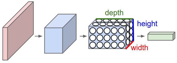
A CNN is made up of Layers. Every layer transforms an input 3D volume to an output 3D volume with some differentiable function that may or may not have parameters. As visualized in the picture above, the red input layer holds the image, so its width and height would be the dimensions of the image, and the depth would be 3 (Red, Green, Blue channels).

Layers in CNN

We use three main types of layers to build CNN architectures: Convolutional Layer, Pooling Layer, and Fully-Connected Layer (exactly as seen in regular Neural Networks). We will stack these layers to form a full CNN architecture.

Convolutional Layer

The convolutional layer is the core building block of a CNN that does most of the computational heavy lifting.

Convolution in CNN is similar to discrete convolution computation, but a bit different (180 degrees rotation). Read this post to understand convolutions and this answer in Zhihu to understand the difference.

Local Connectivity

We connect each neuron in the convolutional layer (blue) to only a local region of the input volume (red). The spatial extent of this connectivity is a hyperparameter called the receptive field of the neuron (equivalently this is the filter size).

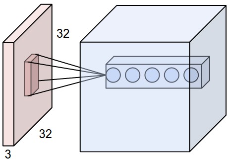
As shown in the picture above, suppose that the input volume (red) has size \([32\times 32 \times3]\), (e.g. an RGB CIFAR-10 image). If the receptive field (or the filter size) is \([5\times5]\), then each neuron in the convolutional Layer (blue) will have weights to a \([5\times5\times3]\) region in the input volume, for a total of \(5\times5\times3 = 75\) weights and \(1\) bias parameter.

Each neuron in the convolutional layer is connected only to a local region in the input volume spatially, but to the full depth (i.e. all color channels). Note, there are multiple neurons (\(5\) in this example) along the depth, all looking at the same region in the input.

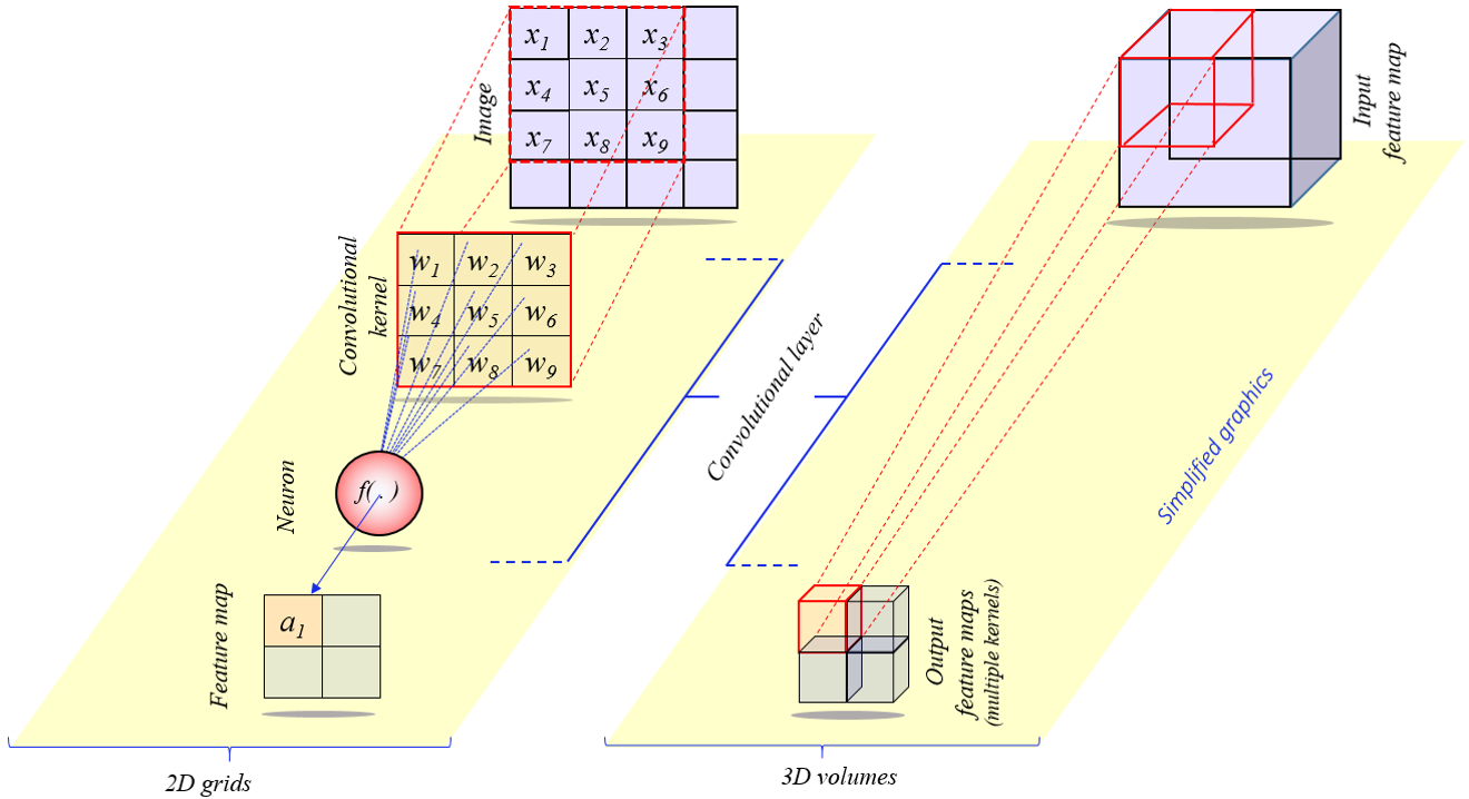
The matrix of weights is called convolutional filter or convolutional kernel, as shown below.

Spatial Arrangement

How many neurons there are in the convolutional layer? How they are arranged? They are controlled by three hyperparameters: the depth, stride and zero-padding.

1. First, the depth of the output volume is a hyperparameter (it is $5$ as shown in the picture above): it corresponds to the number of filters we would like to use, each learning to look for something different in the input. For example, if the first convolutional layer takes as input the raw image, then different neurons along the depth dimension may activate in presence of various oriented edges, or blobs of color. We will refer to a set of neurons that are all looking at the same region of the input as a depth column (or fibre).

2. Second, we must specify the stride with which we slide the filter. When the stride is 1 then we move the filters one pixel at a time. When the stride is $2$ (or uncommonly $3$ or more, though this is rare in practice) then the filters jump $2$ pixels at a time as we slide them around. This will produce smaller output volumes spatially.

3. Third, the size of zero-padding. We can pad the input volume with zeros around the border to control the spatial size of the output volumes (most commonly we use it to make the output volume has the same width and height with the input volume).

Overall, there are four parameters: the receptive field size of the Conv Layer neurons ($F$); the depth of the layer (or the number of filters) ($K$); the stride ($S$); and the amount of zero padding used ($P$) on the border.

Denote the input volume size as $V$. The number of the neurons in the convolutional layer is $(V-F+2P)/S + 1$. We usually set $P=\frac{1}{2}(V \cdot S-V-S+F)$ to ensure that the input volume and output volume have the same size spatially.

Parameter Sharing

Parameter sharing scheme is used to reduce the number of parameters (weights and biases). The assumption is that if one feature is useful to compute at some spatial position \((x_1,y_1)\), then it should also be useful to compute at a different position \((x_2,y_2)\). In other words, denoting a single $2$-dimensional slice of depth as a depth slice (e.g. a volume of size \([64\times64\times100]\) has $100$ depth slices, each of size \([64\times64]\)), we are going to constrain the neurons in each depth slice to use the same weights and bias (different slices use the different weights and bias), which means all $64\times64$ neurons in each depth slice will now be using the same parameters. Each depth slice is computed as a convolution of the neuron’s weights with the input volume (Hence the name: Convolutional Layer).

Note that sometimes the parameter sharing assumption may not make sense. This is especially the case when the input images to a ConvNet have some specific centered structure, where we should expect, for example, that completely different features should be learned on one side of the image than another. One practical example is when the input are faces that have been centered in the image. You might expect that different eye-specific or hair-specific features could (and should) be learned in different spatial locations. In that case it is common to relax the parameter sharing scheme, and instead simply call the layer a Locally-Connected Layer.

Summary

To summarize, the Convolutional Layer:

• Accepts a volume of size $W_1×H_1×D_1$.
• Requires four hyperparameters:
  • depth of the layer (Number of filters) $K$;
  • receptive field size $F$;
  • stride $S$;
  • amount of zero padding $P$.
• Produces a volume of size $W_2×H_2×D_2$, where:
  • $W_2=(W_1−F+2P)/S+1$;
  • $H_2=(H_1−F+2P)/S+1$ (i.e. width and height are computed equally by symmetry);
  • $D_2=K$.
• With parameter sharing, it introduces $F⋅F⋅D_1$ weights per filter, for a total of $(F⋅F⋅D_1)⋅K$ weights and $K$ biases.
• In the output volume, the $d$-th depth slice (of size $W_2×H_2$) is the result of performing a valid convolution of the $d$-th filter over the input volume with a stride of $S$, and then offset by $d$-th bias.
• To keep the conv layer $1$ and layer $2$ have the same size, set $P=(W_1S-S-W_1+F)/2$.

In practice, a common setting of the hyperparameters is $F=3,S=1,P=1$. However, there are common conventions and rules of thumb that motivate these hyperparameters. See the ConvNet architectures section below.

The CNN layers we introduced above are 2D (2 dimensional). There are also 1D and 3D, as shown below. Read this blog for more.

Convolutional dimension	Kernel moves in	Input and output data dimension	Mostly used on
1D	1 direction	2D	Time-Series data
2D	2 directions	3D	Image data
3D	3 directions	4D	3D image data (MRI, CT Scans, Video)

Pooling Layer

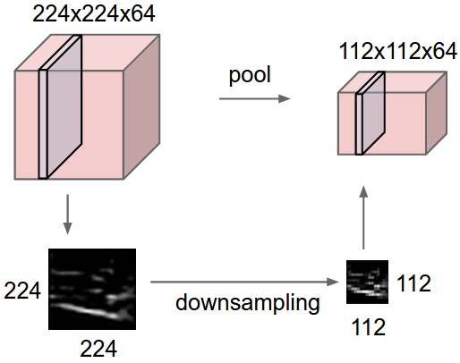
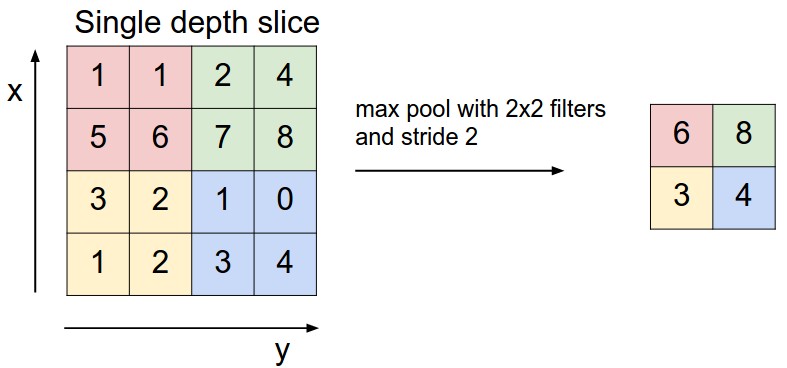
It is common to periodically insert a Pooling layer in-between successive Conv layers. Its function is to progressively reduce the spatial size of the representation to reduce the amount of parameters and computation in the network, and hence to also control overfitting. The Pooling Layer operates independently on every depth slice of the input and resizes it spatially, using the operations like max, average or L2-norm. In practice, max pooling operation normally works better.

The pooling layer:

• Accepts a volume of size $W_1×H_1×D_1$.
• Requires two hyperparameters:
  • receptive field size $F$;
  • stride $S$.
• Produces a volume of size $W_2×H_2×D_2$, where:
  • $W_2=(W_1−F)/S+1$;
  • $H_2=(H_1−F)/S+1$;
  • $D_2=D_1$.
• Introduces zero parameters since it computes a fixed function of the input
• For Pooling layers, it is not common to pad the input using zero-padding.

Pooling sizes with larger receptive fields are too destructive. There are two commonly seen variations of the max pooling layer:

• $F=3,S=2$ (also called overlapping pooling);

• $F=2,S=2$ (more comonly).

Getting rid of pooling. Many people dislike the pooling operation and think that we can get away without it. For example, Striving for Simplicity: The All Convolutional Net proposes to discard the pooling layer in favor of architecture that only consists of repeated CONV layers. To reduce the size of the representation they suggest using larger stride in CONV layer once in a while. Discarding pooling layers has also been found to be important in training good generative models, such as variational autoencoders (VAEs) or generative adversarial networks (GANs). It seems likely that future architectures will feature very few to no pooling layers.

Layer Patterns

The most common form of a ConvNet architecture stacks a few CONV-RELU layers, follows them with POOL layers, and repeats this pattern until the image has been merged spatially to a small size, then follows with fully-connected layers. The last fully-connected layer holds the output, such as the class scores.

INPUT -> [[CONV -> RELU]*N -> POOL?]*M -> [FC -> RELU]*K -> FC

where the * indicates repetition, and the POOL? indicates an optional pooling layer. Moreover, N >= 0 (and usually N <= 3), M >= 0, K >= 0 (and usually K < 3).

We usually prefer a stack of small filter Conv layers to one large receptive field Conv layer. Intuitively, stacking CONV layers with tiny filters as opposed to having one CONV layer with big filters allows us to express more powerful features of the input, and with fewer parameters. As a practical disadvantage, we might need more memory to hold all the intermediate CONV layer results if we plan to do backpropagation.

Example

Example Architecture: In CIFAR-10, images are only of size \([32\times32\times3]\). A simple CNN for CIFAR-10 classification could have the architecture [INPUT -> CONV -> RELU -> POOL -> FC]. In more detail:

• INPUT \([32\times32\times3]\) will hold the raw pixel values of the image, in this case an image of width $32$, height $32$, and with three color channels R,G,B.
• CONV layer will compute the output of neurons that are connected to local regions in the input, each computing a dot product between their weights and a small region they are connected to in the input volume. This may result in volume such as \([32\times32\times12]\) if we decided to use $12$ filters.
• RELU layer will apply an elementwise activation function, such as the $\max(0,z)$ thresholding at zero. This leaves the size of the volume unchanged (\([32\times32\times12]\)).
• POOL layer will perform a downsampling operation along the spatial dimensions (width, height), resulting in volume such as \([16\times16\times12]\).
• FC (i.e. fully-connected) layer will compute the class scores, resulting in volume of size \([1\times1\times10]\), where each of the $10$ numbers correspond to a class score, such as among the $10$ categories of CIFAR-10. As with ordinary Neural Networks and as the name implies, each neuron in this layer will be connected to all the numbers in the previous volume.

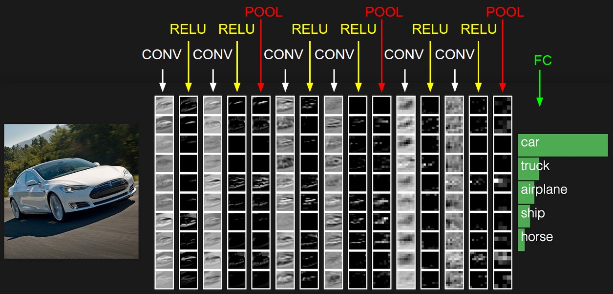
The picture above shows the activations of an example ConvNet architecture. The initial volume stores the raw image pixels (left) and the last volume stores the class scores (right). Each volume of activations along the processing path is shown as a column. Since it’s difficult to visualize 3D volumes, we lay out each volume’s slices in rows. The last layer volume holds the scores for each class, but here we only visualize the sorted top $5$ scores

Summary

• A ConvNet architecture is in the simplest case a list of Layers that transform the image volume into an output volume (e.g. holding the class scores)

• There are a few distinct types of Layers (e.g. CONV/FC/RELU/POOL are by far the most popular)

• Each Layer accepts an input 3D volume and transforms it to an output 3D volume through a differentiable function

• Each Layer may or may not have parameters (e.g. CONV/FC do, RELU/POOL don’t)

• Each Layer may or may not have additional hyperparameters (e.g. CONV/FC/POOL do, RELU doesn’t)

References:

Goodfellow, Ian, Yoshua Bengio, and Aaron Courville. Deep learning. MIT press, 2016.

CS231n Convolutional Neural Networks for Visual Recognition.