In Boosting, we construct a strong predictive algorithm by iteratively layering weak predictive algorithms (weak learners).

A weak learner is one whose error rate is only slightly better than random guessing. The purpose of boosting is to sequentially apply the weak predictive algorithm to repeatedly modified versions of the data, thereby producing a sequence of weak learners: $f_m(x), m = 1, 2, \cdots, M$.

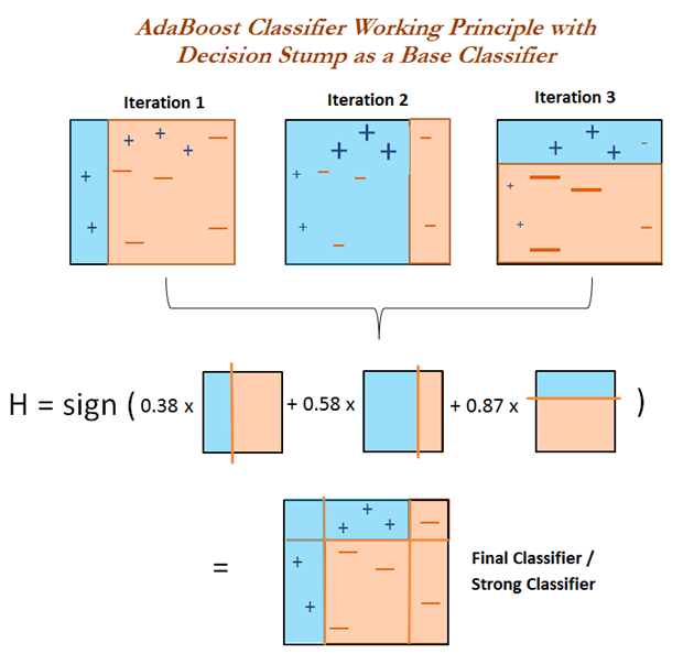
The predictions from all of them are then combined through a weighted majority vote to produce the final prediction:

\[f^{(M)}(x) = \sum_{m=1}^{M} \eta_m f_m(x).\]

Here $\eta_1,\eta_2,\cdots ,\eta_M$ are computed by the boosting algorithm, and weight the contribution of each respective $f_m(x)$. Their effect is to give higher influence to the more accurate learners in the sequence. The data modifications at each boosting step consist of applying weights $w_1,w_2,\cdots, w_N$ to each of the training observations \((x_i,y_i),i=1,2,\cdots,N\).

AdaBoost

AdaBoost, short for Adaptive Boosting, is a basic boosting methods. It can be implemented for both regression and classification problems.

The algorithm below is the AdaBoost.M1 algorithm that used for classification problem.

Algorithm. AdaBoost.M1.

[1] Initialize the observation weights \({w_i}_1 = \frac{1}{N}, i=1,2,\cdots,N\).

[2] For $m = 1$ to $M$, do:

  (a) Fit a classifier $f_m(x)$ to the training data using weights $w_i$;

  (b) Compute \(\text{err}_m = \frac{\sum_{i=1}^{N} {w_i}_m \mathbf{1}(y_i \neq f_m(x_i))}{\sum_{i=1}^{N} {w_i}_m}\);

  (c) Compute \(\alpha_m = \log \big( \frac{1 − \text{err}_m}{\text{err}_m} \big)\);

  (d) Update sample weight \({w_i}_{m+1} = {w_i}_m \cdot \exp\left[\alpha_m \cdot \mathbf{1}(y_i \neq f_m (x_i))\right]\) for all \(i\).

[3] Output $f^{(M)}(x) = \sum_{m=1}^{M} \eta_m f_m(x).$

Boosting Fits an Additive Model

Boosting is a way of fitting an additive expansion in a set of elementary “basis” functions. The philosophy is like Taylor expansion.

Basis function expansions take the form

\[f(x) = \sum_{m=1}^{M} \eta_m b(x; \theta_m),\]

where $\eta_m , m = 1, 2, . . . , M$ are the expansion coefficients, and $b(x; \theta) ∈ \mathbb{R}$ are usually simple basis functions of the multivariate argument $x$, characterized by a set of parameters $\mu$.

In the algorithm AdaBoost.M1. The basis functions are the individual classifiers \(f_m(x) \in \{−1, 1\}\).

Algorithm: Forward Stagewise Additive Modeling.

[1] Initialize $f^{(0)}(x) = 0$.

[2] For $m = 1$ to $M$, do:

  (a) Compute \((\eta_m, \theta_m) = \operatorname*{argmin}_{\eta,\theta} \sum_{i=1}^{N} L\big(y_i, f_{m−1}(x_i) + \eta b(x_i;\theta)\big)\).

  (b) Set $f^{(m)}(x) = f^{(m−1)}(x) + \eta_mb(x;\theta_m)$.

[3] Output $f^{(M)}(x)$.

Suppose $\theta$ is of dimension $p_{\theta}$. In $m$-th step, we need to do optimization with $1+p_{\theta}$ parameters ($\eta_m$ is $1$ dimension and $\theta_m$ is $p_{\theta}$). At the end, $f^{(M)}(x)$ has $M(1+p_{\theta})$ parameters. That is much easier than we do optimization with $M(1+p_{\theta})$ parameters simultaneously: \((\eta, \theta) = \operatorname*{argmin}_{\eta,\theta} \sum_{i=1}^{N} L\big(y_i, f^{(M)}(x_i)\big)\).

AdaBoost.M1 is equivalent to forward stagewise additive modeling using the exponential loss function $L(y, f (x)) = \exp(-y f (x))$. Exponential loss is suitable for classification but not for regression.

Gradient boosting and XGBoost use the gradient descent and Newton’s method respectively to do the step [2] (a) in the algorithm above, and minimize the loss (or objective) function iteratively.

Boosting Trees

Tree ensemble methods (boosting: e.g. GBM, XGBoost, bagging: e.g. random forest) are widely used. Almost half of data mining competition are won by using some variants of tree ensemble methods.

As for CART, a constant $\mu_j$ is assigned to each region $R_j$ and the predictive rule is $x ∈ R_j ⇒ f(x)=\mu_j$.

Thus a tree can be expressed as the additive model form:

\[\text{Tree}(x;Θ) = \sum_{j=1}^{T} \mu_j \mathbf{1}(x \in R_j),\]

with parameters \(Θ = \{R_j , \mu_j\}^T_1\), where \(T\) is the number of leaf nodes and is usually treated as a meta-parameter.

The parameters are found by minimizing the training loss

\[\hat{Θ} = \operatorname*{argmin}_{Θ} \sum_{j=1}^{T} \sum_{x_i \in R_j} L(y_i,\mu_j),\]

It is useful to divide the optimization problem into two parts:

1. Finding \(R_j\): A typical strategy is to use a greedy, top-down recursive partitioning algorithm to find the \(R_j\).
2. Finding \(\mu_j\) given \(R_j\): Given the \(R_j\), often \(\hat{\mu}_j = \frac{1}{\mid R_j\mid} \sum_{x_i \in R_j} y_i\) , which is the mean of the \(y_i\)’s falling in region \(R_j\).

The boosted tree model is a sum of such trees,

\[f^{(M)}(x) = \sum_{m=1}^{M} \text{Tree}(x; Θ_m),\]

induced in a forward stagewise manner (Algorithm: Forward Stagewise Additive Modeling). At each step in the forward stagewise procedure one must solve

\[\hat{Θ}_m = \operatorname*{argmin}_{Θ_m} \sum_{i=1}^{N} L \big(y_i, f^{(m-1)}(x_i) + \text{Tree}(x_i;\Theta_m) \big)\]

for \(\Theta_m = \{ R_{jm}, \mu_{jm} \}_{j=1}^{T_m}\) of the next tree, given the current model $f^{(m-1)}(x)$.

For $m$-th tree, given the regions $R_{jm}$’s ($j=1,\cdots,T_m$), finding the optimal constants $\mu_{jm}$’s in each region is straightforward and easy. However, finding the regions $R_{jm}$’s for the $m$-th tree is difficult. For squared-error loss, a special case, \(\hat{\Theta}_m\) is simply the parameters of the regression tree that best predicts the current residuals \(y_i - f^{(m-1)}(x_i), (i=1, \cdots,N)\).

Note that in boosting methods, especially boosting trees, we can also use bootstrap sample and subset of features like that in random forest to reduce overfitting.

Gradient Boosting

Gradient boosting is based on gradient descent. Instead of minimizing, gradient boosting use the gradient descent to do the step [2] (a) in the algorithm Forward Stagewise Additive Modeling.

We induce a weak regressor or classifier $f_m(x)$ (e.g. a tree $\text{Tree}(x;Θ_m)$) at the $m$-th iteration to fit the negative gradient, which means the predictions (a vector with dimension $n \times 1$) by weak model $f_m(x)$ are as close as possible to the negative gradient.

We want to minimize $L(y_i, f(x_i)), i=1,…N$, where $f$ is the independent variable.

Recall Taylor expansion: $f(x+\Delta x) \approx f(x)+f’(x)\Delta x$. at $m$-th step, we want to minimize the loss function

\[\sum_{i=1}^{N} L\Big(y_i,f^{(m-1)}(x_i)+f_m(x_i)\Big) \approx \sum_{i=1}^{N} \Big[L(y_i, f^{(m-1)}(x_i)) + g_{im} f_m(x_i) \Big].\]

Here \(f_m(x_i)\) should be $-g_{im}$, and \(g_{im} = \frac{∂L(y_i,f^{(m-1)}(x_i))}{∂f^{(m-1)}(x_i)}\) is the gradient.

Thus, we have the iterative formula:

\[f^{(m)}(x_i) = f^{(m-1)}(x_i) + \eta_m f_{m}(x_i) = f^{(m-1)}(x_i) - \eta_m g_{im},\]

where $\eta_m$ is the step size.

If $L(y_i, f^{(m-1)}(x_i))=\frac{1}{2}[y_i-f^{(m-1)}(x_i)]^2$, then the gradient $\frac{∂L(y_i,f^{(m-1)}(x_i))}{∂f^{(m-1)}(x_i)}=f^{(m-1)}(x_i)-y_i$, which is the residual $r_{im}$.

Gradient boosting decision tree (GBDT) is a method when decision tree is applied as the weak learner in gradient boosting.

Algorithm: Gradient Boosting Decision Tree (GBDT) Algorithm.

[1] Initialize \(f^{(0)}(x) = \operatorname*{argmin}_\mu \sum_{i=1}^N L(y_i,\mu)\).

[2] For $m = 1$ to $M$, do:

  (a) For $i = 1,2,…,N$ compute

\[g_{im} = \frac{∂L(y_i,f^{(m-1)}(x_i))}{∂f^{(m-1)}(x_i)}.\]

  (b) Fit a regression tree \(f_m(x)\) to the targets $-g_{im}$’s to get terminal regions $R_{jm},j=1,2,..,T_m$.

  (c) For $j = 1,2,…,T_m$, compute the leaf node prediction $\mu_{jm}$. Now we get a new tree

\[f_m(x) = \text{Tree}(x; \Theta_m) = \sum_{j=1}^{T_m} \mu_{jm}\mathbf{1}(x \in R_{jm}).\]

  (d) Compute step size \(\eta_m = \operatorname*{argmin}_{\eta} \sum_{i=1}^N L\big(y_i,f^{(m-1)}(x_i)+ \eta f_m(x_i) \big)\).

  (e) Update

\[f^{(m)}(x) = f^{(m-1)}(x) + \eta_m f_m(x),\]

    where $f_m(x) = \sum_{j=1}^{T_m} \mu_{jm} \mathbf{1}(x \in R_{jm})$ is a new tree ($m$-th tree).

[3] Output $\hat{f}(x) = f^{(M)}(x)$.

References:

Friedman, Jerome, Trevor Hastie, and Robert Tibshirani. The elements of statistical learning. Vol. 1. No. 10. New York: Springer series in statistics, 2001.

张, 凌寒. “GBDT与XGBoost解析及应用.” 腾讯云, 13 May 2019, cloud.tencent.com/developer/article/1424251.