When there are class imbalance problems, it is necessary to apply some techniques in model training. There are four general classes of techniques: Adjusting prior probabilities, Unequal sample weights, Sampling methods, Ensemble methods.

Adjusting Prior Probabilities

Some models use prior probabilities, such as naive Bayes and discriminant analysis classifiers. Unless specified manually, these models typically derive the value of the priors from the training data. Weiss and Provost (2001) suggest that priors that reflect the natural class imbalance will materially bias predictions to the majority class. Using more balanced priors may help deal with a class imbalance.

Take the insurance data for example, the priors are $6\%$ and $94\%$ for the insured and uninsured, respectively. The predicted probability of having insurance is extremely skewed and adjusting the priors can shift the probability distribution away from small values. For example, new priors of $60\%$ for the insured and $40\%$ for the uninsured in the FDA model (flexible discriminant analysis model with MARS hinge functions) increase the probability of having insurance significantly. With the default cutoff, predictions from the new model have a sensitivity of $71.2\%$ and a specificity of $66.9\%$ on the test set, that is much better than the FDA model with default priors.

However, the new class probabilities did not change the rankings of the customers in the test set and the model has the same area (AUC) under the ROC curve as the previous FDA model. Like the previous tactics for an alternative cutoff, this strategy did not change the model but allows for different trade-offs between sensitivity and specificity.

Unequal Sample Weights

Many of the predictive models for classification have the ability to use case weights where each individual data point can be given more emphasis in the model training phase. For example, AdaBoost creates a sequence of weak learners, each of which apply different case weights at each iteration.

One approach to rebalancing the training set would be to increase the weights for the samples in minority classes.

Denote $r_i$ as the instance weight for the $i$-th instance, the total weighted average loss is then calculated as

\[\frac{1}{\sum_{i=1}^n r_i} \sum_{i=1}^n r_i\text{Loss}(\hat{y}_i, y_i).\]

For many models, this can be interpreted as having identical duplicate data points with the exact same predictor values. Logistic regression, for example, can utilize case weights in this way. This procedure for dealing with a class imbalance is related to the sampling methods discussed in next section.

Sampling Methods

Here we introduce two general sampling approaches: down-sampling (under-sampling) and up-sampling (over-sampling) the data.

Down-Sampling

Down-sampling refers to any technique that reduces the number of samples in majority classes to improve the balance across classes. The most basic down-sampling approach is to randomly sample the majority classes so that all classes have approximately the same size. However, this basic approach may lose information of the original data since many majority class examples are ignored.

There are some advanced down-sampling methods like RUS, NearMiss, ENN, Tomeklink etc..

Up-Sampling

Up-sampling refers to any technique that simulates or imputes additional data points in minority classes to improve balance across classes. The most basic up-sampling approach is to sample the cases from the minority classes with replacement until each class has approximately the same number. However, this basic approach may lead to overfitting since it bring in many duplicate samples.

The synthetic minority over-sampling technique (SMOTE), described by Chawla et al. (2002), synthesizes new cases to up-sample for the minority class, to overcome the overfitting problem posed by random oversampling. There are different methods to synthesizes new cases. For example, we can use the \(K\) nearest neighbors, a data point is randomly selected from the minority class and its $K$ (say $5$) nearest neighbors are determined. We then randomly select a neighbor and synthesize new data point by linear interpolation between the selected data point and neighbor.

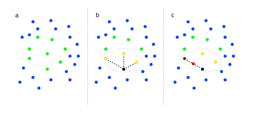
The new synthetic data point is a combination of the predictors (features) of the randomly selected data point and its neighbors. We can also synthesize new data points by interpolation.

There are some extensions to SMOTE that are more selective regarding the examples from the minority class that provide the basis for generating new synthetic examples, like Borderline-SMOTE, Borderline-SMOTE SVM, and Adaptive Synthetic Sampling (ADASYN). The idea is that, the data points that are in a region of the border of decision boundary (where class membership may overlap) are difficult to classify, and we use the difficult minority data points to synthesize new data points.

Borderline-SMOTE uses the \(K\) nearest neighbors to determine whether a minority data point is difficult. Say there are \(K_{+}\) data points in the \(K\) nearest neighbors of a minority data point \(x\), then \(x\) is difficult if \(\frac{1}{2} < \frac{K_{+}}{K} < 1\). Note that \(x\) may be a outlier if \(\frac{K_{+}}{K} = 1\).

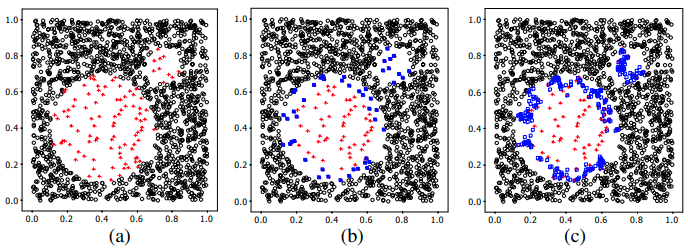
For Borderline-SMOTE SVM, the borderline area is approximated by the support vectors obtained after training a standard SVM classifier on the original training set. Then the minority class support vectors are treated as difficult minority data points.

Adaptive Synthetic Sampling (ADASYN) uses a weighted distribution for different minority class examples according to their level of difficulty in classifying, where more synthetic data is generated for minority class examples that are harder to classify.

Note that when using modified versions of the training set, resampled estimates of model performance can become biased. It should be noted that there is no clear winner among the various sampling methods. Also, different modeling techniques react differently to sampling.

Ensemble Methods

With Unequal Sample Weights

AdaCost, a variant of AdaBoost, introduced by XuYing Liu, et al., is a misclassification cost-sensitive boosting method. When updating sample weights, it adds a cost-adjustment function

\[\beta(i) = \begin{cases} \beta_+(c_i) & \text{if } y_i = f_m (x_i), \\ \beta_-(c_i) & \text{if } y_i \neq f_m (x_i). \end{cases}\]

In the formula above, \(c_i\) is the cost factor and we set it large for minority class samples and small for majority. We require \(\beta_+(c_i)\) to be non-increasing with respect to \(c_i\), \(\beta_-(c_i)\) to be non-decreasing, and both are non-negative.

We then update the sample weights as

\[{w_i}_{m+1} = {w_i}_m \cdot \exp\left[\log \left( \frac{1 − \text{err}_m}{\text{err}_m} \right) \cdot \mathbf{1}\left(y_i \neq f_m (x_i)\right) \cdot \beta(i) \right],\]

for the \(i\)-th sample at the \(m\)-th iteration.

With Down-Sampling

EasyEnsemble and BalanceCascade are introduced by XuYing Liu, et al. to deal with imbalance classification problems by down-sampling and ensemble methods.

EasyEnsemble is similar to bagging. It samples several subsets from the majority class, trains a learner using each of them, and combines the outputs of those learners.

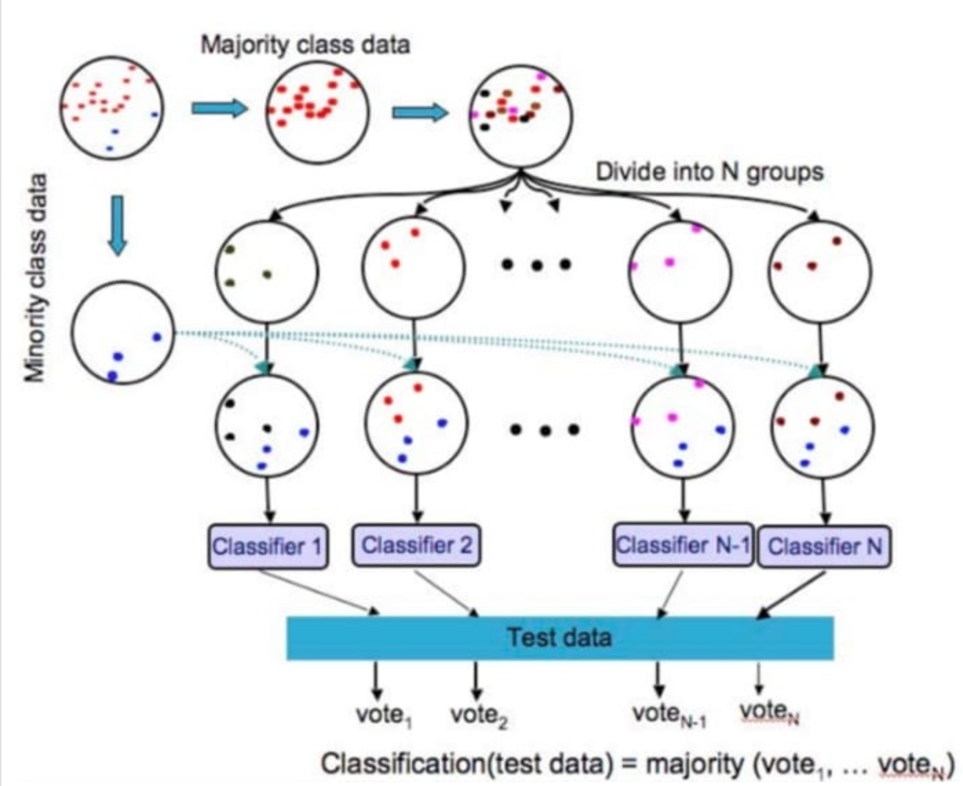
BalanceCascade is a boosting method. It trains the learners sequentially, where in each step the majority class examples which are correctly classified by the current trained learners are removed from further consideration.

References:

Kuhn, M., & Johnson, K. (2013). Remedies for severe class imbalance. In Applied predictive modeling (pp. 419-443). Springer, New York, NY.

Chawla, N., & Bowyer, K., & Hall, L., & Kegelmeyer, W. (2002). SMOTE: Synthetic Minority Over-Sampling Technique. Journal of Artificial Intelligence Research, 16(1), 321–357.

Han, H., Wang, W. Y., & Mao, B. H. (2005, August). Borderline-SMOTE: a new over-sampling method in imbalanced data sets learning. In International conference on intelligent computing (pp. 878-887). Springer, Berlin, Heidelberg.

Brownlee, J. (2020, Jan 17). SMOTE for Imbalanced Classification with Python. Machine learning mastery. Retrieved Oct 23, 2020, from https://machinelearningmastery.com/smote-oversampling-for-imbalanced-classification/.

刘, 芷宁 (2019, Jun 19). 极端类别不平衡数据下的分类问题研究综述. 磐创AI. Retrieved Oct 23, 2020, from https://cloud.tencent.com/developer/article/1448584/.

Lemaitre, G., & Nogueira, F., & Oliveira D., & Aridas C. (2016). Imbalanced-learn API. Imbalanced-learn documentation. Retrieved Oct 23, 2020, from https://imbalanced-learn.readthedocs.io/en/stable/api.html.

Fan, W., Stolfo, S. J., Zhang, J., & Chan, P. K. (1999, June). AdaCost: misclassification cost-sensitive boosting. In Icml (Vol. 99, pp. 97-105).

Liu, X. Y., Wu, J., & Zhou, Z. H. (2008). Exploratory undersampling for class-imbalance learning. IEEE Transactions on Systems, Man, and Cybernetics, Part B (Cybernetics), 39(2), 539-550.