6. Evaluating Model Performance

6.1 For Regression

Mean absolute error (MAE): \(\frac{1}{n} \Vert Y - \hat{Y} \Vert_1 = \frac{1}{n} \sum_{i=1}^{n} \vert y_i - \hat{y}_i \vert\).

Mean squared error (MSE): \(\frac{1}{n} \| Y - \hat{Y} \| _2^2 = \frac{1}{n} \sum_{i=1}^{n} (y_i - \hat{y}_i)^2\).

Root MSE: \(\sqrt{\frac{1}{n} \| Y - \hat{Y} \| _2^2 }= \sqrt{\frac{1}{n} \sum_{i=1}^{n} (y_i - \hat{y}_i)^2}\).

MSE is the most commonly used metric. MAE is more robust and less sensitive to outliers or influential points. However, MAE is not differentiable at the point $y_i-\hat{y}_i = 0$, which is not amenable to numerical optimization.

6.2 For Classification

6.2.1 Loss Functions for Classification

For $K$ classification problem,

Misclassification error: \(\text{Loss}(y_i,\hat{y}_i) = \frac{1}{2} \sum_{k=1}^{K} \mathbf{1}(y_{ik} \neq \hat{y}_{ik} )\).

Cross entropy loss: \(\text{Loss}(y_i,\hat{p}_i) = \sum_{k=1}^K -y_{ik} \log \hat{p}_{ik}\).

In the formula above, $y_i$, $\hat{y}_ {i}$ or $\hat{p}_ i$ is a vector with dimension $K \times 1$; $y_{ik}$, $\hat{y}_ {ik}$ or \(\hat{p}_{ik}\) is the $k$-th element in the vector $y_i$, \(\hat{y}_i\) or \(\hat{p}_i\); $y_{ik}=1$ if the $i$-th observation is of class $k$, and $y_{ik}=0$ otherwise; \(\hat{y}_{ik}=1\) if the $i$-th observation is classified to be the class $k$ by the model, and \(\hat{y}_{ik}=0\) otherwise; \(\hat{p}_{ik}\) is the estimated probability of the $i$-th observation is of class $k$.

Cross entropy loss for binary classification problem: $ \frac{1}{n} \sum_{i=1}^n \big[ -y_i \log \hat{p}_i - (1-y_i) \log(1-\hat{p}_i) \big]$.

Cross-entropy loss measures the difference between two probability distributions, but not the distance, because it is asymmetric. Cross-entropy loss is differentiable, and hence more amenable to numerical optimization.

6.2.2 Metrics for Classification

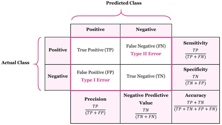
Precision \(=\frac{TP}{TP+FP}\) is the fraction of true positive instances among the predicted positive instances. Recall (Sensitivity) \(=\frac{TP}{TP+FN}\) is the fraction of the total amount of positive instances that were actually retrieved.

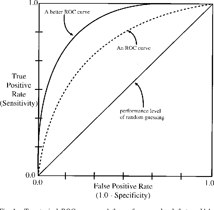
If we have the estimated probabilities \(\hat{p}_1, \cdots ,\hat{p}_n\), then \(\hat{y}_i = \text{sign}(\hat{p}_i > \text{threshold})\). We can change the threshold from \(1\) to \(0\) and plot the TPR (true positive rate, or sensitivity, or recall) v.s. FPR (false positive rate, or \(1-\) specificity). When the threshold is \(1\), all cases are classified as negative, and \(\text{TPR} = \text{FPR} = 0\). When the threshold is \(0\), all cases are classified as positive, and \(\text{TPR} = \text{FPR} = 1\).

The plot is known as ROC (receiver operating characteristic) curve. The AUC (area under curve) is the area under the ROC curve. The larger of the AUC, the better of the classification model.

Note that the metrics are not the loss functions.

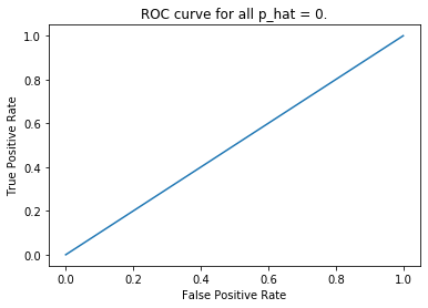
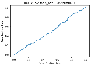
If we predict all cases as positive (or negative), we get the straight ROC curve, and the AUC is $0.5$. Also, if we generate estimated probabilities randomly as \(\hat{p}_i \overset{\text{i.i.d.}}{\sim} \text{Uniform}(0,1)\), the corresponding ROC curve is also very close to a straight line. As simulated below.

from random import random
from sklearn.metrics import roc_curve
import matplotlib.pyplot as plt

test = [0] * 900 + [1] * 100
predict1 = [0] * 1000
predict2 = [random() for _ in range(1000)]
fpr1, tpr1, _ = roc_curve(test, predict1)
fpr2, tpr2, _ = roc_curve(test, predict2)

plt.plot(fpr1, tpr1)
plt.xlabel('False Positive Rate')
plt.ylabel('True Positive Rate')
plt.title('ROC curve for all p_hat = 0.')
plt.show()

plt.plot(fpr2, tpr2)
plt.xlabel('False Positive Rate')
plt.ylabel('True Positive Rate')
plt.title('ROC curve for p_hat ~ Uniform(0,1).')
plt.show()

There are more metrics like F1 score and Cohen’s kappa coefficient, etc..

7. Regularization

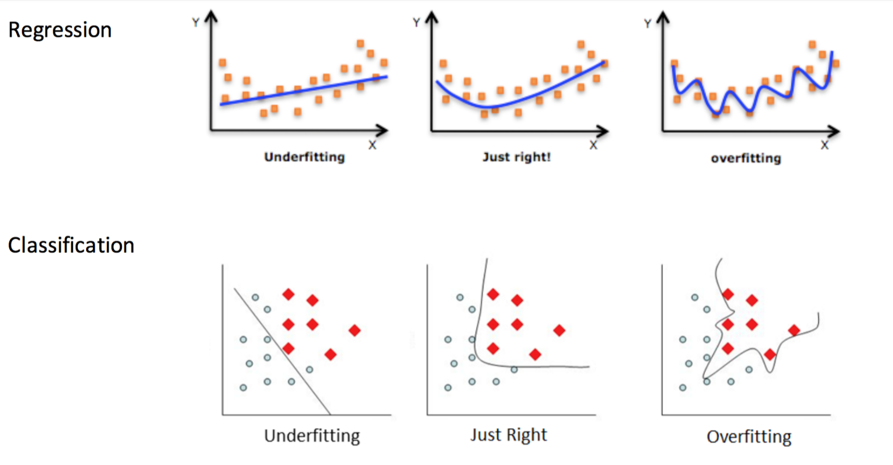
7.1 Overfitting

If a model learned too much noise in the training data, it tends to be overfitting, and the training error is much lower than the test error. Overfitting often happens for flexible models. An overfitted model has low bias but high variance. Regularization discourages learning a more complex or flexible model, so as to reduce overfitting.

7.2 L1 and L2 Regularization

L1-norm regularization: $\text{Loss} + \lambda \Vert w \Vert_1$.

L2-norm regularization: $\text{Loss} + \lambda \Vert w \Vert _2^2$.

The hyperparameter $\lambda$ depends the regularization strength. Note: a hyperparameter is a parameter whose value is set before the learning process begins. By contrast, the values of other parameters are derived via training.

Linear regression with L1-norm is LASSO and L2-norm is ridge regression.

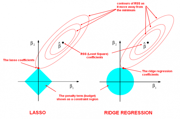
L1-norm shrinks some coefficients (or weights) to $0$ and produces sparse coefficients, so it can be used to do feature selection. The sparsity makes the model more robust and also more computationally efficient when doing prediction.

L2-norm encouraging the model to use all of its inputs a little rather than some of its inputs a lot. It is differentiable so it has an analytical solution and can be calculated efficiently when training model. Notice that during gradient descent parameters update, using the L2-norm regularization ultimately means that the parameter is decayed linearly: W -= lambda * W towards zero.

8. Optimization

Assume we have the objective function

where $\theta$ is a vector of dimension \(d\) that contains the parameters of predictive model $f(\cdot)$, $L(\cdot)$ is the loss function, and $\Omega(\cdot)$ is the regularization term.

Our objective is to minimize the objective function with respect to $\theta$: $\theta^* = \underset{\theta}{\text{argmin }} \text{Obj}(Y,X,\theta)$.

Sometimes the objective function is convex with respect to \(\theta\), and also the exact solution of \(\theta\) is available by solving \(\frac{\partial \text{Obj}(Y,X,\theta)}{\partial \theta} = 0\), like linear regression, then applying gradient based methods is not a must. However, in some cases, like the sample size or the number of features is very large, even when these two conditions are satisfied and the unique exact solution is available, it is also worth to use gradient based methods since it is usually computationally cheaper. For example, we can use gradient descent to get the solution of linear regression, when the data matrix \(X\) is huge and the computation of the exact solution \(\hat{\beta} = (X^TX)^{-1}X^TY\) is too expensive to afford.

However, the conditions of convex and exact solution are not satisfied in most cases, and we need to apply gradient based methods to find the minimum of objective function. In the following sections, let’s first introduce the gradient descent and Newton’s method as iteratively minimizing the local Taylor approximation to the objective function, and then some advanced gradient based methods.

8.1 Gradient Descent

We perform $\theta^{(t)} = \theta^{(t-1)} + \Delta\theta^{(t)}$ iteratively until the objective function converges. Denote $\Delta \theta = \alpha \mathbf{u}$, where $\alpha$ is a non-negative scalar (length of $\Delta\theta$) and $\mathbf{u}$ is a unit vector (direction of $\Delta\theta$).

By the Taylor polynomial of degree one,

where $\gamma$ is the angle between $\mathbf{u}$ and $\text{Obj}’(\theta)$.

We want to find the unit vector $\mathbf{u}$ that minimize $\text{Obj}(\theta + \alpha\mathbf{u})$. Obviously, the minimizer $\mathbf{u}$ should have the opposite direction of $\text{Obj}’(\theta)$ that make $\text{cos}(\gamma)=-1$, then we have \(\mathbf{u} = \frac{-\text{Obj}'(\theta)}{\| \text{Obj}'(\theta) \|}\).

Thus, we have

where \(\eta_{t} = \frac{\alpha^{(t-1)}}{\| \text{Obj}'(\theta^{(t-1)}) \|}\) is called the step size or learning rate.

8.2 Newton’s Method

We use the Taylor polynomial of degree two to decompose the objective function,

$\text{Obj}’’(\theta)$ is the Hessian matrix that contains all second order partial derivatives:

To find the minimum of the objective $\text{Obj}(\theta + \Delta\theta)$, we take its first derivative with respect to $\Delta\theta$, then equate it with $0$ and solve for $\Delta\theta$,

Thus, we have

where $\eta_{t}$ is the step size or learning rate.

By using the Taylor polynomial of degree two, Newton’s method is more accurate than gradient descent, thus needs less iterations. On the other hand, it is more computationally expensive. Computing the inverse of the Hessian matrix costs \(O(d^3)\) time, which is very expensive, and we can try Quasi-Newton methods.

8.3 Proximal Gradient Descent

If the function is not differentiable everywhere (e.g. L1 norm, ReLU), we can use the sub-gradient of the function to update the parameters. However, for LASSO, we usually use the proximal gradient descent, rather than the sub-gradient descent. For ReLU, we usually simply set the sub-gradient as \(0\) or \(1\) when it comes to the zero point (indifferentiable). We don’t use proximal gradient descent for ReLU because we need a (sub-)gradient to backprobagate.

References:

James, Gareth, et al. “Statistical Learning.” An introduction to statistical learning. Vol. 112. New York: springer, 2013.

Friedman, Jerome, Trevor Hastie, and Robert Tibshirani. The elements of statistical learning. Vol. 1. No. 10. New York: Springer series in statistics, 2001.