Representational Power

Kolmogorov Arnold Representation theorem states that any continuous function $f$ can be exactly represented by (possible infinite) sequence of addition, multiplication and composition with functions that are universal (do not depend on $f$).

It can be shown (e.g. see Approximation by Superpositions of Sigmoidal Function, or this intuitive explanation) that given any continuous function $f(x)$ and some $ϵ>0$, there exists a Neural Network $\hat{f}(x)$ with one hidden layer (with a reasonable choice of non-linearity, e.g. sigmoid) such that $ \forall x, \mid f(x)−\hat{f}(x) \mid < \epsilon$. In other words, the one hidden layer neural network can approximate any continuous function.

Despite the fact that their representational power is theoretically equal, in practice, as we increase the size and number of layers in a Neural Network, the capacity of the network increases. That is, the space of representable functions grows since the neurons can collaborate to express many different functions.

Units

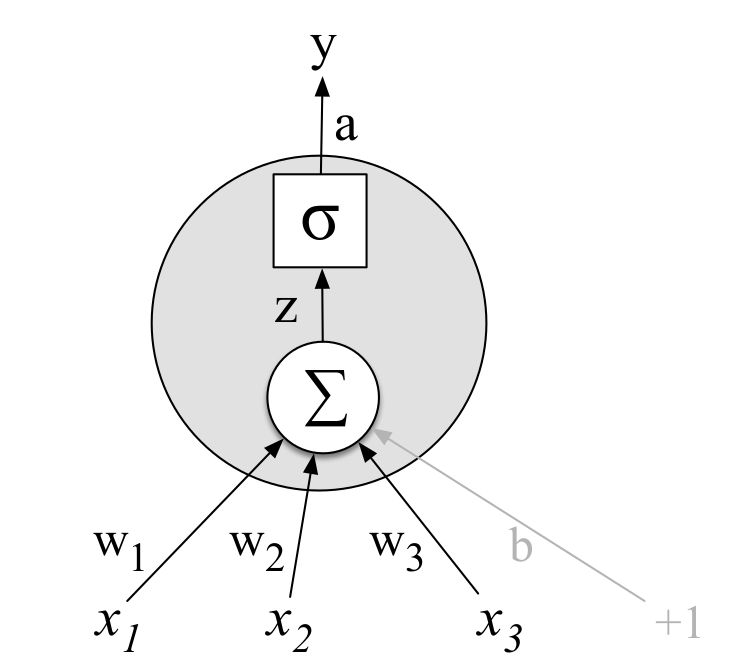
Single Unit

Taking a weighted sum of its inputs and then applying a activation function. $\sigma(z)=\sigma(w^Tx+b)$, where the vector $w$ is called weight, the scalar $b$ is called bias, the function $\sigma(\cdot)$ is called activation function.

For linear regression, $\sigma(z)=z$. For logistic regression, $\sigma(z)=\frac{1}{1+e^{-z}}$.

Activation Functions

Activation functions are usually non-linear. If they are all linear, then we simply get the linear combination of the inputs, and that is the same as linear regression.

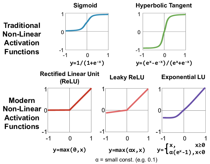
Sigmoid, Tanh

They both have S-shape curve. Note that \(\text{Tanh}(z) = 2\cdot\text{Sigmoid}(2z) - 1\).

\[\text{Sigmoid: }\sigma(z)=\frac{1}{1+e^{-z}}; \text{ Tanh: } \sigma(z)=\frac{e^z-e^{-z}}{e^z+e^{-z}}.\]

A major drawback of sigmoid and tanh is the vanishing gradient problem. When the neuron’s activation saturates at either tail of \(0\) or \(1\), the gradient at these regions is almost zero. During backpropagation, this (local) gradient will be multiplied to the gradient of this gate’s output for the whole objective. Therefore, if the local gradient is very small, it will effectively “kill” the gradient and almost no signal will flow through the neuron to its weights and recursively to its data.

Another drawback of sigmoid is that its outputs are not zero-centered. This is not a problem of tanh, and that’s why tanh is usually better than sigmoid. This is a drawback since neurons in later layers of processing in a Neural Network would be receiving data that is not zero-centered. This could introduce undesirable zig-zagging dynamics in the gradient updates for the weights. It has less severe consequences compared to the saturated activation problem above.

Here is why zig-zagging. Say a layer has inputs \(x_i\)’s, which are the outputs of the previous layer. If the activation function of the previous layer is sigmoid, then \(x_i>0\). In current layer, we have \(z=\sum_iw_ix_i + b\). Now we compute the gradients of the parameters \(w_i\)’s in the current layer.

\[\frac{\partial \text{Loss}}{\partial w_i} = \frac{\partial \text{Loss}}{\partial z} \frac{\partial z}{\partial w_i} = \frac{\partial \text{Loss}}{\partial z} x_i.\]

Since \(x_i>0\) for all \(i=1,2,\cdots\), the gradients \(\frac{\partial \text{Loss}}{\partial w_i}\) for all $i$ have the same sign (positive or negative) as \(\frac{\partial \text{Loss}}{\partial z}\).

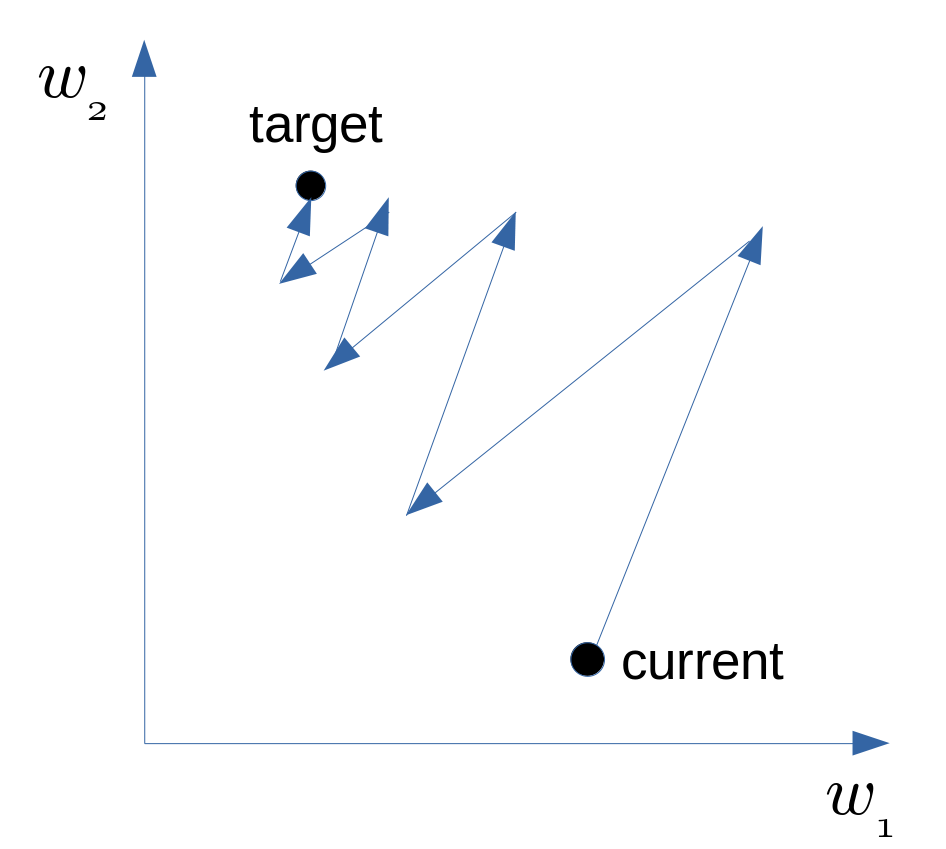
For example, say there are two parameters \(w_1,w_2\), and the gradients of them are always of the same sign. That means \(w_1\) and \(w_2\) increase or decrease simultaneously in the parameters updates, and it also means we can only move roughly in the direction of northeast or southwest in the parameter space. If our goal happens to be in the northwest or southeast side of our current position, then it will cost a lot to move to our target position, as shown below.

ReLU, Leaky ReLU, ELU

ReLU is the short for rectified linear units, and ELU is short for exponential linear unit.

\[\text{ ReLU: } \sigma(z)=\max(z,0); \\ \text{ Leaky ReLU: } \sigma(z)=\max(z, \alpha z)= \begin{cases} \alpha z & \text{ for } z<0, \\ z & \text{ for } z\geq 0; \end{cases} \\ \text{ ELU: } \sigma(z)=\max(z, \alpha (e^z-1))= \begin{cases} \alpha (e^z-1) & \text{ for } z<0, \\ z & \text{ for } z\geq 0. \end{cases}\]

where $\alpha$ is a small positive number. e.g. $0.01$.

Pros of ReLU: 1. It greatly accelerate the convergence of stochastic gradient descent compared to the sigmoid/tanh functions. It is due to its linear, non-saturating form; 2. Computation is easier.

Cons of ReLU: 1. ReLU units can be fragile during training and can “die”. For example, a large gradient flowing through a ReLU neuron could cause the weights to update in such a way that the neuron will never activate on any datapoint again. If this happens, then the gradient flowing through the unit will forever be zero from that point on. However, with a lower learning rate this is less frequently an issue; 2. The range of ReLu is \([0, \infty )\). This means it can blow up the output of the activation function.

Leaky ReLUs are one attempt to fix the “dying ReLU” problem. Instead of the function being zero when $x<0$, a leaky ReLU will instead have a small positive slope (of $0.01$, or so). However, it not always have benefits.

Pros of ELU: ELU is smooth at the point \(0\) and becomes smooth slowly until its output equals to \(-α\), whereas ReLU or leaky ReLU is sharp at the point \(0\).

Cons of ELU: 1. 2. same as that of ReLU; 3. more computationally expensive since it involves exponential operations.

Pros	ReLU	Leaky ReLU	ELU
Non-saturating	✓	✓	✓
Computationally easy	✓	✓	✗
Smooth	✗	✗	✓

Cons	ReLU	Leaky ReLU	ELU
Fragile (dead neurons)	✓	✗	✗
Blow up the output	✓	✓	✓

Maxout

\[\text{ Maxout: } \sigma(z_{1},\cdots,z_{k})=\max(w_1^Tx + b_1,\cdots,w_k^Tx + b_k).\]

A maxout unit can learn a piecewise linear, convex function with up to $ k $ pieces. Maxout units can thus be seen as learning the activation function itself rather than just the relationship between units. With large enough $ k, $ a maxout unit can learn to approximate any convex function with arbitrary fidelity. In particular, a maxout layer with two pieces can learn to implement the same function of the input $ x $ as a traditional layer using the ReLU, the absolute ReLU, or the leaky or parametric ReLU, or it can learn to implement a new function. For example, for ReLU we have $\max(w^Tx+b, 0^Tx+0)$. However, a maxout unit have $k$ times of the number of parameters for every single unit, leading to a high total number of parameters.

What neuron type should I use? Use the ReLU non-linearity, be careful with your learning rates and possibly monitor the fraction of “dead” units in a network. If this concerns you, give Leaky ReLU or Maxout a try. Never use sigmoid. Try tanh, but expect it to work worse than ReLU/Maxout.

Feed-Forward Neural Networks

A feedforward network is a multilayer network in which the units are connected with no cycles; the outputs from units in each layer are passed to units in the next higher layer, and no outputs are passed back to lower layers. Simple feedforward networks have three kinds of nodes: input units, hidden units, and output units. The core of the neural network is the hidden layer formed of hidden units, each of which is a neural unit. In the standard architecture, each layer is fully-connected.

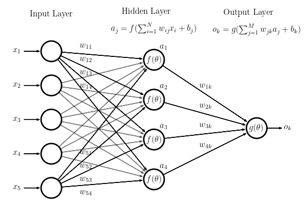
Let’s assume there are $n^{[l-1]}$ hidden units in the hidden layer $l-1$ and $n^{[l]}$ units in the layer $l$. Denote the output of the layer \(l-1\) (it is also the input of the layer \(l\)) as $a^{[l-1]} \in \mathbb{R}^{n^{[l-1]}}$. In the layer \(l\), denote the weight matrix as $W^{[l]} \in \mathbb{R}^{n^{[l]}\times n^{[l-1]}}$, bias vector as $b^{[l]}\in\mathbb{R}^{n^{[l]}}$, activation function as \(\sigma^{[l]}(\cdot)\), then the output of the layer \(l\) is

\[a^{[l]} = \sigma^{[l]}(W^{[l]} a^{[l-1]} + b^{[l]}) \in \mathbb{R}^{n^{[l]}}.\]

For example, the picture below shows a fully-connected layer (layer 2). There are two units in layer 1 and three units in layer 2.

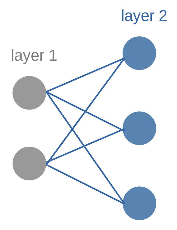
The mathematical expression of this plot is (dimension is labeled under the symbol):

\[\underset{3\times1}{a^{[2]}} = \sigma^{[2]}(\underset{3\times2}{W^{[2]}} \underset{2\times1}{a^{[1]}} + \underset{3\times1}{b^{[2]}}).\]

For $K$-class classification problems, we usually apply softmax function at output layer : \(\sigma (\mathbf {z} )_k={\frac {e^{z_k}}{\sum _{l=1}^{K}e^{z_{l}}}}{\text{ for }}k=1,\dotsc ,K {\text{, where }}\mathbf {z} =(z_{1},\dotsc ,z_{K})\in \mathbb {R} ^{K}.\)

The output layer thus gives the estimated probabilities of each output node (corresponds to each class). If the number of classes is too large, it may be helpful to use Hierarchical Softmax.

We traditionally don’t count the input layer when numbering layers, but do count the output layer.

Model Ensembles

One approach to improving the performance of neural networks is to train multiple independent models, and then average their predictions. As the number of models in the ensemble increases, the performance typically monotonically improves (though with diminishing returns). The improvements are more dramatic with higher model variety in the ensemble.

There are a few approaches to forming an ensemble:

• Same model, different initializations. Use cross-validation to determine the best hyperparameters, then train multiple models with the best set of hyperparameters but with different random initialization. The danger with this approach is that the variety is only due to initialization.
• Top models discovered during cross-validation. Use cross-validation to determine the best hyperparameters, then pick the top few (e.g. 10) models to form the ensemble. This improves the variety of the ensemble but has the danger of including suboptimal models. In practice, this can be easier to perform since it doesn’t require additional retraining of models after cross-validation.
• Different checkpoints of a single model. If training is very expensive, some people have had limited success in taking different checkpoints of a single network over time (for example after every epoch) and using those to form an ensemble. Clearly, this suffers from some lack of variety, but can still work reasonably well in practice. The advantage of this approach is that is very cheap.
• Running average of parameters during training. We average the states of the network over last several iterations. You will find that this “smoothed” version of the weights over last few steps almost always achieves better validation error. The rough intuition to have in mind is that the objective is bowl-shaped and your network is jumping around the mode, so the average has a higher chance of being somewhere nearer the mode.

One disadvantage of model ensembles is that they take longer to evaluate on test example.

Tips

Regression and Classification

As for neural networks, the L2 loss (MSE) for regression problem is much harder to optimize than a more stable loss such as Softmax for classification problem. Intuitively, it requires a very specific property from the network to output exactly one correct value for each input (and its augmentations). The L2 loss is less robust because outliers can introduce huge gradients.

When faced with a regression task, first consider if it is absolutely necessary. Instead, have a strong preference to discretizing your outputs to bins and perform classification over them whenever possible. For example, if you are predicting star rating for a product, it might work much better to use 5 independent classifiers for ratings of 1~5 stars instead of a regression loss.

If you’re certain that classification is not appropriate, use the L2 but be careful: For example, the L2 is more fragile and applying dropout in the network (especially in the layer right before the L2 loss) is not a great idea.

Use GPU

GPUs are used heavily in deep learning, because GPUs are well suited for parallel computing, and neural networks are embarrassingly parallel.

References:

Goodfellow, Ian, Yoshua Bengio, and Aaron Courville. Deep learning. MIT press, 2016.

CS231n Convolutional Neural Networks for Visual Recognition.