The contents in this post are mainly excerpted from ¹ (thanks Jurafsky and Martin for this excellent textbook), and also ².

Inability of RNNs to Maintain Critical Memory

Although RNNs can theoretically capture long-term dependencies, however, in practice, it is quite difficult to train RNNs to do this. In other words, it is hard to train RNNs to be able to make use of information distant from the current point of processing.

However, it is often that the distant information is critical to many language applications. To see this, consider the following example. Given a sentence “The flights the airline was cancelling were full”, it is straightforward to assign a high probability to “was” following “airline”, but assigning an appropriate probability to “were” is quite difficult, not only because the plural “flights” is quite distant, but also because the intervening context “airline” involves singular constituents.

One reason for the inability of RNNs to carry forward critical information is that the weights \(U, W\) that determine the values in the hidden layer, are being asked to perform two tasks simultaneously: provide information useful for the current decision, and updating and carrying forward information required for future decisions. Second is that the simple RNNs may suffer from gradient vanishing problem.

To address these issues, more complex network architectures have been designed to manage context over time. More specifically, the networks needs to learn to forget information that is no longer needed and to remember information required for decisions still to come.

Long Short Term Memory (LSTM)

Long short term memory (LSTM) ³ network was introduced by Hochreiter and Schmidhuber in 1997. It divides the context management problem into two sub-problems: removing information no longer needed from the context, and adding information likely to be needed for later decision making.

LSTMs accomplish this by first adding an explicit context layer to the architecture in addition to the usual recurrent hidden layer, and through the use of specialized neural units that make use of gates to control the flow of information into and out of the units that comprise the network layers.

The gates in an LSTM share a common design pattern; each consists of a feedforward layer with input word and past hidden state as the inputs, followed by a sigmoid activation function, followed by a pointwise multiplication with the layer being gated. The choice of the sigmoid as the activation function arises from its tendency to push its outputs to either $0$ or $1$. Combining this with a pointwise multiplication has an effect similar to that of a binary mask. Values in the layer being gated that align with values near $1$ in the mask are passed through nearly unchanged; values corresponding to lower values are essentially erased.

Now let’s introduce three gates and two generation cells in the context layer of LSTM networks, and see mathematically how an LSTM uses \(h_{t−1}\) and \(x_t\) to generate the next hidden state \(h_t\).

Forget Gate

The purpose of the forget gate is to delete information from the past memory (context) \(c_{t-1}\) that is no longer needed. The forget gate computes a weighted sum of the previous state’s hidden layer $h_{t-1}$ and the current input \(x_t\) and passes that through a sigmoid \(\sigma(\cdot)\) to produce the indicator $f_t$.

\[f_t = \sigma (W_{f}x_t + U_f h_{t-1}).\]

We then use $f_t$ as an indicator to gate the past memory (context) \(c_{t-1}\).

New Memory Generation

A new memory \(\tilde{c}_t\) is the consolidation of a new input word \(x_t\) with the past hidden state \(h_{t-1}\). The new memory is the actual information we need to extract from the previous hidden state and current inputs. Here we use the tanh function because it produces zero-centered outputs.

\[\tilde{c}_t = \text{tanh}(W_{c}x_t + U_{c}h_{t-1}).\]

Input Gate

The purpose of the input gate is to select information from new memory (context). The input gate uses the input word $x_t$ and the past hidden state \(h_{t-1}\) to produce the indicator \(i_t\).

\[i_t = \sigma (W_{i}x_t + U_{i}h_{t-1}).\]

We then use \(i_t\) as an indicator to gate the new memory \(\tilde{c}_t\).

Final Memory Generation

We use the forget gate to remove the information from past memory (context) \(c_{t-1}\) that is no longer required, and use the input gate \(i_t\) to select the information from new memory \(\tilde{c}_t\). Both removing and selecting are achieved through pointwise multiplication. It then sums these two results to produce the final memory \(c_t\).

\[c_t = f_t \odot c_{t-1} + i_t \odot \tilde{c}_t.\]

Output/Exposure Gate

The purpose of the output gate \(o_t\) is to select information from final memory $c_t$ to be the new hidden state \(h_t\). The final memory $c_t$ contains a lot of information that is not necessarily required to be saved in the new hidden state \(h_t\). The output gate still uses \(x_t\) and \(h_{t-1}\) to produce the indicator \(o_t\).

\[o_t = \sigma (W_o x_t + U_oh_{t-1}).\]

New Hidden State Generation

Finally, we use \(o_t\) as an indicator to gate the final memory \(c_t\) to produce the new hidden state \(h_t\).

\[h_t = o_t \odot \text{tanh}(c_t).\]

Summary for LSTM

Here is the architecture of an LSTM.

An LSTM accepts as input the context layer \(c_{t-1}\), and hidden layer \(h_{t-1}\) from the previous time step, along with the current input vector \(x_t\). It then generates updated memory (context) \(c_t\) and hidden vectors \(h_t\) as output.

In the context layer of an LSTM, the new memory generation cell generates new memory \(\tilde{c}_t\), and the forget gate and input gate produce indicators \(f_t\) and \(i_t\) to gate past memory \(c_{t-1}\) and new memory \(\tilde{c}_t\) respectively. After that, the final memory generation cell generates final memory \(c_t\) based on the indicators, past memory, and new memory. Finally, the output gate produces indicator \(o_t\) to gate final memory \(c_t\), and then we generate new hidden state \(h_t\).

Gated Recurrent Unit (GRU)

The Gated Recurrent Unit (GRU) ⁴ was introduced by Cho et al. in 2014. It is motivated by LSTM unit but is much simpler to compute and implement.

We have 8 sets of weights to learn (i.e., the \(U\) and \(W\) for each of the 4 gates within each unit) in LSTM, whereas with simple recurrent units we only had 2. Training these additional parameters imposes a much significantly higher training cost. GRU eases this burden by dispensing with the use of a separate context vector, and by reducing the number of gates to 2 — a reset gate and an update gate.

Reset Gate

The purpose of the reset gate is to decide which aspects of the previous hidden state \(h_{t-1}\) are relevant to the current hidden state and what can be ignored.

\[r_t = \sigma (W_{r}x_t + U_r h_{t-1}).\]

New Memory Generation

A new memory (or called an intermediate representation for the new hidden state \(h_t\)) \(\tilde{h}_t\) is the consolidation of a new input word \(x_t\) with the past hidden state \(h_{t−1}\).

\[\tilde{h}_t = \text{tanh}(Wx_t + U(r_t \odot h_{t-1})).\]

Update Gate

The purpose of the update gate is to determine which aspects of the new memory \(\tilde{h}_t\) will be used directly in the new hidden state \(h_t\) and which aspects of the previous state \(h_{t-1}\) need to be preserved for future use.

\[z_t = \sigma (W_z x_t + U_z h_{t-1}).\]

New Hidden State Generation

Finally, the new hidden state \(h_t\) is generated by using the indicator \(z_t\) to interpolate between the past hidden state \(h_{t-1}\) and the new memory \(\tilde{h}_t\).

\[h_t = z_t h_{t-1} + (1-z_t) \tilde{h}_t.\]

When \(z_t=1\), we have \(h_t = h_{t-1}\), which is similar to identity mapping by shortcut in ResNet.

Summary for GRU

Summary

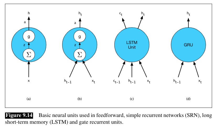
Although LSTM unit and GRU are much more complex than basic recurrent unit, we can still maintain modularity of LSTM unit and GRU and to easily experiment with different architectures. To see this, the following figure illustrates the inputs and outputs associated with each kind of unit.

References: