The contents in this post are excerpted from the paper “Hotspot: Anomaly localization for additive kpis with multi-dimensional attributes” ¹.

Introduction

This paper proposes an approach, called HotSpot, to automatically localize the root cause, one (or more) combination of attribute values in multiple dimensions. In this paper, our measure (or called KPI) is page view (PV).

Problem Definition

Important Terms

A vector of the distinct attribute value combination is called an element in this paper, denoted as \(e=(p, i, d, c)\), where \((p \in \mathrm{P} \text{ or } p=*)\), \((i \in \mathrm{I} \text{ or } i=*)\), \((d \in \mathrm{D} \text{ or } d=*)\), and \((c \in \mathrm{C} \text{ or } c=*)\), \(*\) is the wildcard. Here, the “distinct” means that an element can be \((\text{Beijing}, \text{Mobile})\) or \((*, \text{Mobile})\), but cannot be \((\text{Beijing } \lor \text{ Shanghai}, \text{Mobile})\). Denote the real value according an element \(e\) as \(v(e)\). Denote the collection of all the most fine-grained elements as \(\text{LEAF} = \{e \mid e=(p,i,d,c), p\neq*, i\neq*, d\neq*, c\neq*\}\).

As shown in Figure 1, the elements of \(\text{LEAF}\) constitute a 4-d data cube. The cuboid is denoted as \(B_{i}\) (\(i\) can be an arbitrary combination of \(P, I, D\) and \(C\)), e.g., \(B_{P}\) is a 1-d cuboid and \(B_{P, I, D}\) is a 3-d cuboid. The element set of a cuboid \(B_{i}\) is denoted as \(E(B_i)\), e.g., \(E\left(B_{P}\right)=\{e \mid e=(p, *, *, *), p \neq *\}\), \(E\left(B_{P, I, D}\right)=\{e \mid e=(p, i, d, *), p \neq *, i \neq *, d \neq *\}\), \(\text{LEAF} = E\left(B_{P, I, D, C}\right)\).

Moreover, we structure the cuboids and label layer IDs for them, as shown in Figure 2. In addition, we say \(B_{P}\) or \(B_{I}\) is a father cuboid of \(B_{P, I}\), and \(B_{P, I}\) is a child cuboid of \(B_{P}\) or \(B_{I}\). Accordingly, the elements of the cuboids, such as \((p, *, *, *)\left(\in E\left(B_{P}\right)\right)\) and \((p, i, *, *)\left(\in E\left(B_{P, I}\right)\right)\), also have the father-and-child relationships.

We denote \(e^{\prime}=\left(p^{\prime}, i^{\prime}, d^{\prime}, c^{\prime}\right)\) as a descendant of \(e=(p, i, d, c)\) iff \(\left(e \neq e^{\prime}\right)\) and \(\left(p^{\prime}=p\right.\) or \(\left.p=*\right)\) and \(\left(i^{\prime}=i\right.\) or \(i=*\) ) and \(\left(d^{\prime}=d\right.\) or \(d=*\) ) and \(\left(c^{\prime}=c\right.\) or \(\left.c=*\right) . \operatorname{Desc}(e)=\left\{e^{\prime} \mid e^{\prime}\right.\) is a descendant of \(\left.e\right\}\). \(\operatorname{Desc}^{\prime}(e)=\left\{e^{\prime} \mid e^{\prime}=\left(p^{\prime}, i^{\prime}, d^{\prime}, c^{\prime}\right) \in L E A F, e^{\prime} \in \operatorname{Desc}(e)\right\}\). If \(e \in L E A F\), then PV value \(v(e)\) is directly measured. Otherwise,

\[v(e)=\sum _{e'\in Desc'(e)}{v(e')}\]

e.g.,

\[v(\text{Beijing},*,*,*) = \sum _{j,k,h}{v(\text{Beijing}, i_{j}, d_{k}, c_{h})}, \\ \text{Total}~PV=v(*,*,*,*)\!=\!\sum _{i,j,k,h}{v(p_{i}, i_{j}, d_{k}, c_{h})}.\]

Problem Statement

The additive KPI (with multi-dimensional attributes) anomaly localization problem is to identify the cuboid and its elements that most potentially have caused the anomalous change of the total KPI value.

As an example shown in Table 4, each cuboid contains a set of elements, i.e., \(E(BP)=\{(\text{Beijing},∗),(\text{Shanghai},∗),(\text{Guangdong},∗)\}\), \(E(BI)=\{(∗, \text{Mobile}),(∗,\text{Unicom})\}\), \(\text{LEAF} = E(BP,I)=(\text{Beijing}, \text{Mobile}) , (\text{Shanghai}, \text{Mobile}) , (\text{Guangdong}, \text{Mobile}) ,\) \((\text{Beijing}, \text{Unicom}) , (\text{Shanghai}, \text{Unicom}) , (\text{Guangdong}, \text{Unicom})\). \(v(p,i)\) are shown in the cells of the table, e.g., \(v(\text{Beijing}, \text{Mobile})=20\), \(v(\text{Beijing},∗)=30\).

The problem of anomaly localization for additive KPIs can be restated as follows:

Effectively and efficiently identify the most potential root cause, i.e., a subset of elements of one specific cuboid \(B_i\), for a total KPI value anomaly. The root cause set \(\text{RSet} \subseteq E(B_i)\).

Note that this definition allows the multiple elements within the same cuboid as the root cause set. For instance, a root cause can be \(\text{RSet}=\{(\text{Beijing},∗),(\text{Shanghai},∗)\}\). However, this definition excludes the cases where there are simultaneous root causes in multiple cuboids, which is extremely rare in reality. Also note that we only deal with the case where total KPI value is anomalous.

Challenges

There are mainly two challenges for our anomaly localization problem.

1. How to measure the potential of an attribute combination set to be the root cause?

2. How to design the searching and pruning strategy to localize the root cause from a huge search space?

Core Idea and Overview

For challenge 1, we propose Potential Score as the metrical function.

For challenge 2, we apply Monte Carlo Tree Search (MCTS) algorithm and hierarchical pruning strategy.

Recall that the root cause set \(\text{RSet}\) is one of the \(2^n-1\) subsets of a cuboid with \(n\) elements inside.

Design of HotSpot

HotSpot searches the sets of cuboids layer by layer, i.e., from layer \(1\) to layer \(L\) (\(L\) is the number of layers). For each cuboid of a given layer, HotSpot applies MCTS to find its subset with the largest potential score (ps), which is called best set (abbreviated \(\text{BSet}\)) of this cuboid. When going from a layer to the next layer, hierarchical pruning is used. We repeat this process until layer \(L\) is searched, or the root cause set \(\text{RSet}\) (\(ps(\text{RSet}) > PT\)) is obtained, where \(PT\) (\(ps\) Threshold) is a threshold that we think it is large enough to be regarded as the root cause set when a set with a \(ps > PT\). The final output \(\text{RSet}\) is the \(\text{BSet}\) with the largest \(ps\) among all \(\text{BSet}\)s generated by the algorithm.

Potential Score

Our idea for this Potential Score is based on the following intuition: when the KPI value at a root cause element changes, all its descendant LEAF elements’ KPI values also change accordingly.

Ripple Effect

Generally, when the value of a root cause element increases or decreases, it obeys the ripple effect property as follows:

Let \(x\) denote an element that is not in \(\text{LEAF}\), i.e., \(x \notin \text{LEAF}\). Let \(x_{i}^{\prime}\) denote the descendant elements of \(x\) in \(\text{LEAF}\), i.e., \(x_{i}^{\prime} \in \operatorname{Desc}^{\prime}(x)\). When the PV value of \(x\) changes by \(h(x)\), i.e., \(h(x)=f(x)-v(x), x_{i}^{\prime}\) will get its share of \(h(x)\) according to the proportions of their forecast values, i.e.,

\[v(x'_{i}) = f(x'_{i}) - h(x) \times \dfrac {f(x'_{i})}{f(x)}, ~(f(x)\neq 0).\]

Potential Score

The ripple effect reveals how a root cause set affects many other elements’ values. Therefore, to measure the potential of a set to be the root cause, we propose to 1) assume that the set \(S\) is the root cause, 2) deduce new PV values of the descendant elements in \(\text{LEAF}\) based on the ripple effect, and 3) compare all the actual PV values with the newly deduced PV values of \(\text{LEAF}\) elements. The closer the two kinds of values are, the more potential the set has to be the root cause set.

If \(y_{i} \in \text{LEAF}\), we denote the newly deduced PV values of an assumed root cause set \(S\) with \(a(y_{i})\). if \(y_{i} \notin \operatorname{Desc}^{\prime}(S)\), \(a(y_{i})=f(y_{i})\). Let \(\vec{a}\) be the vector of \(a(y_{i})\), i.e., \(\vec{a}=[a(y_{1}), a(y_{2}), a(y_{3}), \ldots, a(y_{n})]\), where \(n\) is the element count of \(\text{LEAF}\). Similarly, let \(\vec{v}=[v(y_{1}), v(y_{2}), v(y_{3}), \ldots, v(y_{n})], \vec{f}=[f(y_{1}), f(y_{2}), f(y_{3}), \ldots, f(y_{n})]\). Then we define the Potential Score \((p s)\) of a set \(S\):

\[\text { Potential Score }=\max \left(1-\frac{d(\vec{v}, \vec{a})}{d(\vec{v}, \vec{f})}, 0\right),\]

where \(d(\vec{u}, \vec{w})\) represents the distance of the vectors \(\vec{u}\) and \(\vec{w}\). Here we adopt the Euclidean distance:

\[d(\vec{u}, \vec{w})=\sqrt{\sum_{i}\left(u_{i}-w_{i}\right)^{2}}\]

The potential score of a set ranges from 0 to 1, i.e., \([0,1]\). If a set has a higher score, it will be considered to have higher potential to be the root cause.

When two element sets have the same potential score, we follow a “succinctness” principle. i.e., the one with less number of element wins, either following the Occam’s razor principle or because the elements of one set are collectively the ancestors (preferred as root cause) of those in the other. E.g. \(\{(\text{Beijing},*)\}\) is more succinct than \(\{(\text{Beijing},\text{Mobile})\}\), and is also more succinct than \(\{(\text{Beijing},*), (\text{Shanghai},*)\}\).

MCTS Algorithm

For a given cuboid \(B\), we apply MCTS to obtain the best set (the subset with the largest potential score of this cuboid). Suppose there are n elements in \(E(B)\). The search space within \(B\) for the root cause set is \(2^n-1\), which apparently can be very large for a large \(n\).

MCTS is a heuristic method for searching optimal decisions in a given domain by taking random samples in the decision space and building a search tree according to the results from existing random examples. At the very high-level, MCTS tries to balance the exploitation along those promising branches and the exploration along those unexplored branches.

In MCTS, each node represents a state \(s\) (the root can be regarded as \(\varnothing\)). An action space \(A(s)\) contains all the legal actions that can be taken at \(s\). The algorithm can move from one state \(s\) to another by taking a legal action, named \(a \in A(s)\), via the edge \((s, a)\). There can be variables associated with an edge, used by the algorithm to indicate the “value” of taking action \(a\) at state \(s\).

We adopt MCTS to our anomaly localization problem in a cuboid as follows. We first calculate \(p s(e)\) for each \(e\) in this cuboid, and rank all \(e\) according to \(p s(e)\). Each state \(s\) corresponds to the candidate root cause set \(S(s)\) that is currently being explored. \(N(s)\) is the number of times \(s\) has been visited. We setup three variables for each edge \((s, a) . N(s, a)\) is visit count, i.e., the number of times that edge \((s, a)\) has been visited. \(p s(S(s))\) is the potential score of set \(S(s)\). Suppose \(s\) transitions to \(s^{\prime}\) following \((s, a)\). Then edge \((s, a)\) ‘s action value \(Q(s, a)=\max _{u \in\left\{s^{\prime}\right\} \cup \operatorname{descendent}\left(s^{\prime}\right)} p s(S(u))\), which equals the maximum potential score of \(s^{\prime}\) and its descendant nodes in the tree. \(Q(s, a)\) is initialized to be \(p s(S(s))\) for each \(s\). (It is initialized as \(0\) in this reproduction)

Selection

The goal of this step is to select a node from the current state tree to be expanded. Each time when this step is executed, the tree traversal always starts with the root state.

Assume that we have advanced to the current state \(s\) in this selection step. If all the actions in \(A(s)\) have been visited in previous iterations, then an action \(a\) is selected from the set of available actions \(A(s)\) by using the Upper Confidence Bound (UCB) algorithm, shown as below:

\[a = \mathop {\arg\max}_{a \in A(s)} \left\{Q(s, a) + C \sqrt{\frac{\ln N(s)}{N(s, a)}}\right\}. \tag{8}\]

\(Q(s, a)\) is the value of taking the move \(a\). The higher the value of \(Q(s, a)\), the larger the chance of move \(a\) is selected in this selection step, which is the exploitation mechanism in MCTS. The second part of the equation is just the standard UCB mechanism for exploration. The balance between exploitation and exploration can be changed by modifying \(C\). A commonly used value of \(C\) is \(\sqrt{2}\), which we choose in this paper, or it can be chosen empirically in practice.

In case there is an action \(a \in A(s)\) that has not been explored at all, equation 8 cannot be applied since \(N(s, a)=0\). Instead, we assign a probability of taking unvisited actions to be \(R=\left(1-Q\left(s, a_{\max }\right)\right)\), where \(a_{\max }=\arg \max _{a \in A(s) \cap N(s, a) \neq 0} Q(s, a)\).

The selection step starts at the root of the tree, and stops when a leaf state is chosen according to equation 8 or an unvisited action is selected. E.g., in Figure 4(a) along with the bold edges, the selection step stops when the leaf state \(\left\{e_{1}, e_{3}\right\}\) is selected.

Expansion

After a state \(s\) is selected in the selection step, we then expand the Monte Carlo Tree by adding a new node \(s^{\prime}\), where \(S\left(s^{\prime}\right)=S(s) \cup\left\{e^{*}\right\}\) and \(e^{*}=\arg \max _{e \in\left\{e_{1}, e_{2}, \ldots, e_{n}\right\}-S(s)} p s(e)\). We choose \(e^{*}\) to have the largest \(p s(S)\) value of the remaining elements rather than choosing \(e^{*}\) randomly.

For example, in Figure 4(b), \(s\) (where \(S(s)=\left\{e_{1}, e_{3}\right\}\) ) is selected, and then \(e^{*}=e_{4}\) is added to get \(s^{\prime}\) where \(S\left(s^{\prime}\right)=\left\{e_{1}, e_{3}, e_{4}\right\}\).

Evaluation

To initialize the new node after expansion (e.g., \(\left\{e_{1}, e_{3}, e_{4}\right\}\) in Figure 4(c)), we calculate its \(p s, Q\) and \(N\).

Backup

Action values \(Q\) and visit count \(N\) on all nodes along path from \(s^{\prime}\) to the root are updated, as illustrated by the bold arrows in Figure 4(b). Recall the definition of \(Q\), along the path, we update the \(Q\) of a father only when the child’s \(Q\) is greater than the father’s.

Localizing the root cause set in a cuboid. We apply MTCS in each cuboid, for which we iteratively perform the above four steps until at least one of the following three conditions occur:

1. A best set is found, i.e., \(\text{BSet} = S\) if \(ps(S) \geq PT\);
2. All the available nodes of the set are expanded;
3. The iteration time is greater than a maximum number \(M\), which is configured empirically.

Under both the second and third terminating conditions, if we have not obtained a set whose \(ps\) is greater than \(PT\), we will return the \(\text{BSet}\) with the greatest \(ps\) as the \(\text{RSet}\).

Hierarchical Pruning

In order to further reduce the search space for the cuboids in higher layers, HotSpot applies a hierarchical pruning strategy. The basic idea is that, HotSpot searches the cuboids layer by layer, i.e., from layer \(1\) to layer \(L\). After searching a lower layer, it prunes some elements in the higher layers that is unlikely to be root cause elements.

For each cuboid \(B\) of layer \(l\) \((1 \leq l < L)\), we can obtain the best sets (the subset with the largest potential score of this cuboid) \(\text{BSet}_{l,B}\) using the MCTS algorithm. Our intuition is as follows. If an element \((p_1,i_1,∗,∗)\) in layer \(l+1\) has a high potential score, its father elements \((p_1,∗,∗,∗)\) and \((∗,i_1,∗,∗)\) in layer \(l\) will also have a relatively high potential score. Therefore, if a father element has a very low potential score, each of the children elements is unlikely to be a root cause element. As a result, if an element in layer \(l\) is not in \(\text{BSet}_{l,B}\), HotSpot chooses to prune all its children elements.

We take an example in Table 7 and illustrate our hierarchical pruning approach in Figure 5. Suppose we are in layer 1, and the best sets obtained using MCTS are \(\text{BSet}_{1, B_{P}}=\{(\text{Fujian}, *),(\text{Jiangsu}, *)\}\) with \(p s\left(\text{BSet}_{1, B_{P}}\right)=0.50\), and \(\text{BSet}_{1, B_{I}}=\{(*, \text{Mobile}),(*, \text{Unicom})\}\) with \(ps\left(\text{BSet}_{1, B_{I}}\right)=0.32\). When searching cuboids in layer 2, we prune the elements \((\text{Zhejiang}, \text{Unicom})\) and \((\text{Zhejiang}, \text{Unicom})\) because their father element \((\text{Zhejiang}, *)\) is not in the \(\text{BSets}\) of layer 1. Therefore, we only need to search the remaining four elements for \(B_{P, I}\). This way, the number of potential sets will be reduced from \(63\) to \(15\) (\(2^{6}-1\) to \(2^{4}-1\)). Then using MCTS again in layer 2, we obtain the \(\text{RSet} = \text{BSet}_{2, B_{P, I}} = \{(\text{Fujian}, \text{Mobile}), (\text{Jiangsu}, \text{Unicom}) \}\), where \(ps(\text{BSet}_{2,B_{P, I}})=1\).

The Overall Algorithm

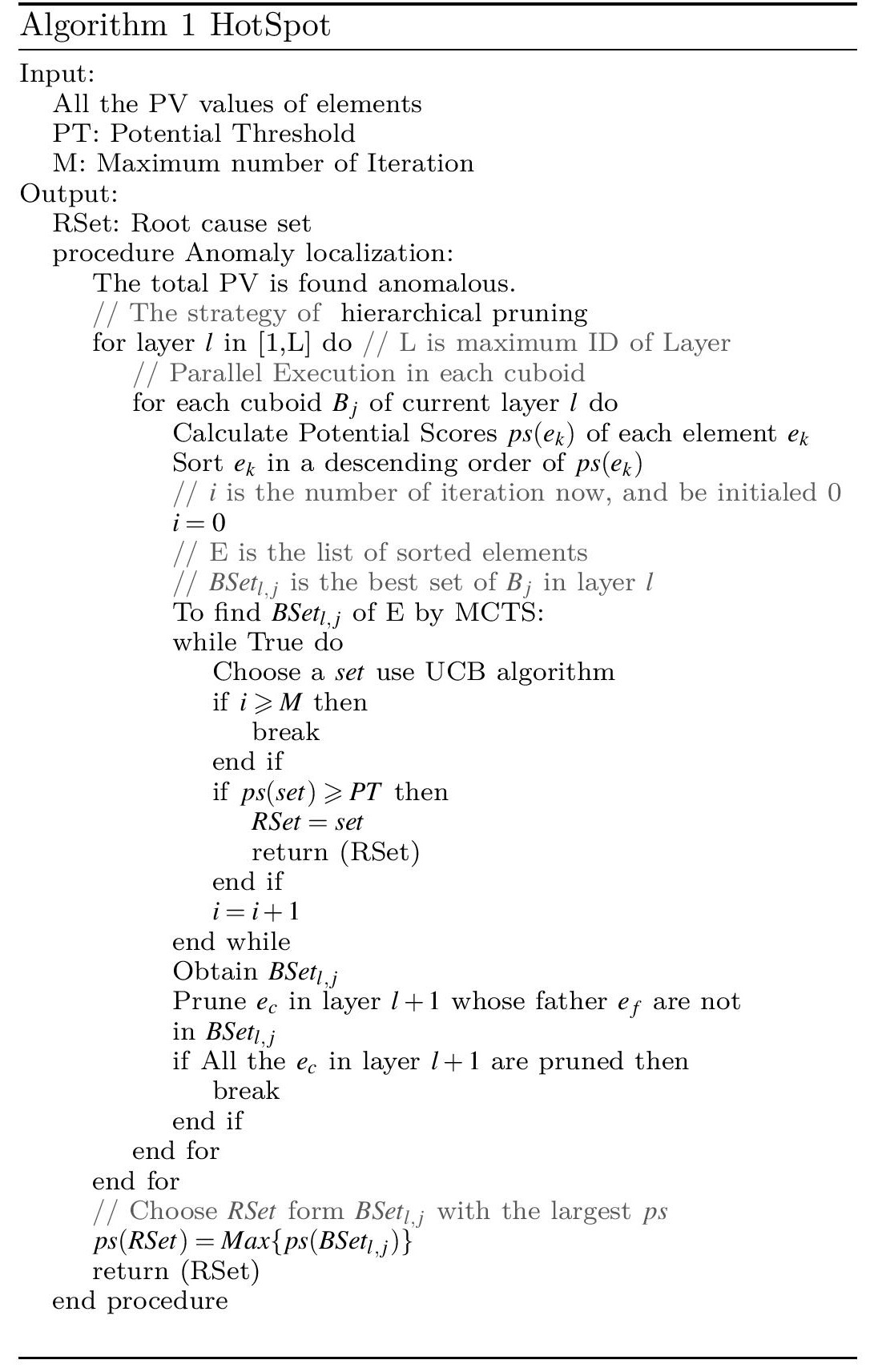
HotSpot takes the PV values of elements, a potential threshold \(PT\) and a maximum iteration number \(M\) as inputs. It starts with layer 1. For each cuboid of a given layer, HotSpot applies MCTS to find its best set. When going from a layer to the next layer, hierarchical pruning is used. We repeat this process until layer \(L\) is searched, or the root cause set \(\text{RSet}\) (\(ps(\text{RSet})>PT\)) is obtained. The final output \(\text{RSet}\) is the the \(\text{BSet}\) with the greatest \(ps\) among all \(\text{BSet}\) generated by the algorithm.

Reference: