The contents in this post are excerpted from the paper “iDice: Problem Identification for Emerging Issues” ¹.

Introduction

We formulate the problem of identifying emerging issues as a pattern mining problem: given a volume of customer issue reports over a period of time, the goal is to search for an attribute combination that isolates the entire multi-dimensional time series dataset into two partitions: one showing a significant increase of issue volume, and the other not showing such an increase. As the number of attribute combinations could be huge, we design several pruning techniques to significantly reduce the search space.

Motivation

An Example

Sometimes the number of issue reports associated with a certain attribute combination could suddenly increase, i.e. an emerging issue could occur. We call such an attribution combination Effective Combination.

Challenge

The dataset of issue reports can be treated as an combination of multi-dimensional data and time series data. Most of the closed itemset approaches only handle multi-dimensionality without considering the temporal property. They cannot detect the change point at which the volume of issue reports significantly increases.

Problem Formulation

Effective Combinations

Because issue report data could contain a large number of attribute combinations, the challenge is to effectively identify the effective combinations from all the possible combinations.

As illustrated in Figure 2. Each node denotes an attribute combination, each edge denotes a subset-superset relationship.

For two attribute combinations \(X\) and \(Y\), if the data containing \(X\) is also included in the data containing \(Y\), we call \(X\) a subset of \(Y\) and \(Y\) a superset of \(X\). For example, ABC is a subset of AB and AC.

Requirements

The author have identified the following requirements for an effective combination:

• Impactful: An effective combination should associate with an emerging issue that corresponds to a relatively large number of issue reports.

• Reflecting changes: The volume of issue reports associated with the identified attribute combination should exhibit a significant burst after the change point, while the volume of reports associated with other attribute combinations does not exhibit the same burst along time.
• Less redundant: The identified attribute combinations should be compact and concise.

The Proposed Approach

In order to effectively reduce the search space, we have designed the following pruning strategies according to the requirements described in Section 3.2:

• Impact based pruning. We adopt an impact based strategy to remove the attribute combinations associated with small numbers of issue reports.
• Change Detection based pruning. We prune off the attribute combinations that exhibit small or no changes in issue volume.
• Isolation power based pruning. We use this strategy to remove the possible redundancy in the identified effective combinations.

Impact based Pruning

In our implementation, we use the BFS (Breadth-first Search) based closed itemset mining approach. We ignore the time stamp information of the issue reports, and apply the BFS-based closed itemset mining algorithm on the entire dataset.

If one attribute combination has no sufficient volume, it is obvious that all its subsets do not have enough volume either. Thus we can directly remove this attribute combination together with all its subsets.

Change Detection based Pruning

For each closed itemset obtained after impact-based pruning, we check whether the corresponding volume of reports has a significant increase. To achieve so, we consider the time stamp information of the data and build time series data for the closed itemsets. Each data point in the time series denotes the volume of reports that contains the corresponding closed itemsets at a particular time stamp. We then apply change detection algorithm to detect the change points (i.e. the points where issue bursts occur) in the time series data.

In our implementation, we adopt GLR (Generalized Likelihood Ratio) as the change detection algorithm. Change detection can be formulated as a hypothesis-testing problem. Suppose the values of a time series fit a distribution \(\theta_0\), if there is a change, the values during the change region conform to another distribution \(\theta_1\). Here, the hypothesis \(H_0\) corresponds to “no change”, and \(H_1\) corresponds to “change”.

GLR maintains a threshold. Given a few continuous data points, if the sum of their logarithm-likelihood-ratio is greater than the threshold, these continuous data points are detected as a change region. The first point of the continuous data points is deemed as the change point. For the time series data without any change points, the corresponding attribute combinations will be pruned.

Isolation Power based Pruning

As discussed in Section 3, an effective combination should be able to isolate the attribute combinations that exhibit changes from the other combinations that do not. This property can help us further remove the possible redundancy in the obtained itemsets. To achieve so, we propose the notion of Isolation Power:

\[\begin{aligned} I P(X) &=-\frac{1}{\overline{\Omega_{a}}+\overline{\Omega_{b}}}\left(\overline{X_{a}} \ln \frac{1}{P(a \mid X)}+\overline{X_{b}} \ln \frac{1}{P(b \mid X)}\right.\\ &\left.+\left(\overline{\Omega_{a}}-\overline{X_{a}}\right) \ln \frac{1}{P(a \mid \bar{X})}+\left(\overline{\Omega_{b}}-\overline{X_{b}}\right) \ln \frac{1}{P(b \mid \bar{X})}\right). \end{aligned}\]

Let $ S_{X} $ be the time series data corresponding to the attribute combination $ X, X_{a} $ denotes the volume of time series data in $ S_{X} $ during the change region of $ X $, and $ X_{b} $ denotes the volume of time series data in $ S_{X} $ before the change point of $ X . \Omega_{a} $ denotes the entire volume during the change region of $ X $, and $ \Omega_{b} $ denotes the entire volume before the change point of $ X $. All $ \bar{*} $ denote the mean value of the corresponding time series. Also:

\[P(a \mid X)=\frac{\bar{X}_{a}}{\bar{X}_{b}+\bar{X}_{a}}, P(b \mid X)=\frac{\bar{X}_{b}}{\bar{X}_{b}+\bar{X}_{a}}, \\ P(a \mid \bar{X})=\frac{\bar{\Omega}_{a}-\bar{X}_{a}}{\bar{\Omega}_{a}+\bar{\Omega}_{b}-\bar{X}_{b}-\bar{X}_{a}}, \\ P(b \mid \bar{X})=\frac{\bar{\Omega}_{b}-\bar{X}_{b}}{\bar{\Omega}_{a}+\bar{\Omega}_{b}-\bar{X}_{b}-\bar{X}_{a}}.\]

The proposed Isolation Power is based on the idea of Information Entropy. As discussed in Section 3 and illustrated by Figure 2, the entire set of attribute combinations form a lattice, and every node in the lattice can split the dataset into two parts: the issue reports that contain the attributes, and the reports that do not contain the attributes. If an attribute combination is an effective combination, all its subset nodes in the lattice exhibit significant increases in the same change region, but its sibling nodes do not. Therefore, an effective combination is the node that can exactly split the entire dataset into two parts: with and without a significant increase.

According to the information theory, the overall entropy of two datasets (e.g., \(A\) and \(B\)) where each dataset (\(A\) or \(B\)) contains samples with an identical property (e.g., all of them exhibit increases, or all of them do not exhibit increases) is much smaller than the entropy of two datasets where samples with different properties are mixed together. Based on this concept, we calculate Isolation Power to mimic the calculation of entropy.

During the search process, if the current set has a higher isolation power than its direct supersets and subsets, then the current set is an effective attribute combination, satisfying the requirements for effective combinations described in Section 3. In this case, all its subsets will not be searched. In this way, we can reduce search space using the Isolation Power measure. Considering a simple example with three attribute combinations:

\[X=\{\text{Country}=\text{India}\} \\ Y=\{\text{Country}=\text{India}; \text{TenantType}=\text{Edu}; \text{DataCenter}=\text{DC6}\} \\ Z=\{\text{Country}=\text{India}; \text{TenantType}=\text{Edu}; \text{DataCenter}=\text{DC6}; \text{Package}=\text{Lite}\}\]

If \(Y\) has a higher isolation power than its subset \(Z\) and superset \(X\), \(Y\) will be considered and \(Z\) and \(X\) will be removed from the search space.

Result Ranking

In real-world scenarios, we may obtain a set of effective combinations from the data. We rank the effective combinations according to their relative significance. We adopt a score similar to Fisher distance for the ranking:

\[R=p_{a} * \ln \frac{p_{a}}{p_{b}}\]

In the above equation, $ p $ denotes the ratio: $ p=\frac{V_{X t}}{V_{t}} $, where $ V_{X t} $ denotes the volume of current effective combination during a time period $ t $ and $ V_{t} $ denotes the total volume during $ t $. $ p_{a}, p_{b} $ are the ratios during the detected change region and before the detected change point respectively.

In our implementation, we prune away the attribute combinations whose \(R\) score is lower than a cutoff threshold (which is empirically set to $1.0$ in our implementation).

Finally, we rank the remaining attribute combinations and output them as the effective combinations.

The Overall Algorithm

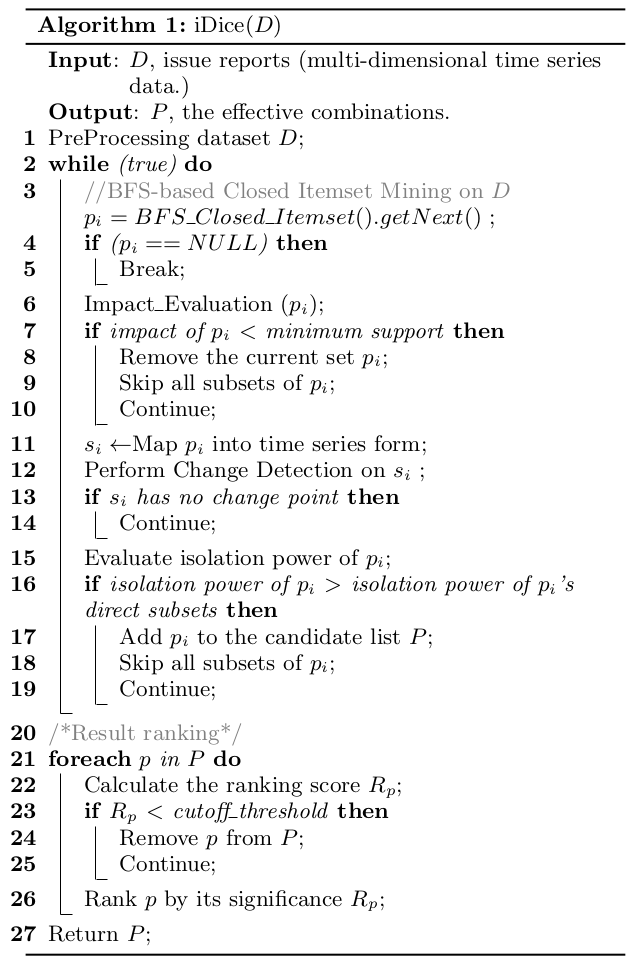
For each closed itemset \(p_i\) returned by the BFS (Breadth First Search) based closed itemset mining process, iDice performs Impact-based pruning (lines 6-10), Change Detection based pruning (lines 11-14), and Isolation Power based pruning (lines 15-19). These steps prune away attribute combinations and reduce the search space, making it possible to identify effective combinations from a large number of attribute combinations. Lines 21 to 26 denote the result ranking part of iDice.

Reference: