
Intro to SVM
For a binary classification problem, a basic idea is that finding a hyperplane in sample space to seperate the samples in two different classes. Any hyperplane in space \(\mathbb{R}^p\) can be expressed as
\[\{x \in \mathbb{R}^p : w^Tx + b = 0\},\]for some \(w \in \mathbb{R}^p, b \in \mathbb{R}\). Denote this hyperplane as \((w,b)\).
Suppose \(y_i \in \{-1,1\}\). If the hyperplane can seperate the samples, then we have
\[\begin{cases} w^Tx_i + b \geq 1, &\text{if } y_i=1, \\ w^Tx_i + b \leq -1, &\text{if } y_i=-1. \end{cases}\]Denote the two parallel hyperplanes as
\[\begin{aligned} & H_1 = \{x \in \mathbb{R}^p : w^Tx + b = 1\}, \\ & H_2 = \{x \in \mathbb{R}^p : w^Tx + b = -1\}. \end{aligned}\]\(H_1\) and \(H_2\) are parallel because \(H_1 \cap H_2 = \emptyset\). We want to make these two hyperplanes separate the data points, and also maximize the margin between them.
The margin between \(H_1\) and \(H_2\) is \(\frac{2}{\| w \|}\).
Proof:
We first prove that, for any \(x_1\in\mathbb{R}^p\), the distance between the point \(x_1\) and the hyperplane \((w,b)\) is \(\frac{\mid w^Tx_1+b \mid}{\| w \|}\).
For any two points \(x_2,x_3\) on the hyperplane \((w,b)\), \(x_2-x_3\) is a vector on \((w,b)\), then we have \(w^T(x_2-x_3)=0\), which means the vector \(w\) is perpendicular to \((w,b)\). Denote \(x_0\) as the projective point of \(x_1\) on \((w,b)\), then the distance between \(x_1\) and \((w,b)\) is \(\|x_1-x_0\|\). The vector \(x_1-x_0\) is perpendicular to \((w,b)\), then we can express it as \(x_1 - x_0 = \|x_1-x_0\|\frac{w}{\|w\|}\). The distance \(\|x_1-x_0\| = \sqrt{(x_1 - x_0)^T(x_1-x_0)} = \sqrt{\|x_1-x_0\| \frac{w^T}{\|w\|} (x_1 - x_0)} = \sqrt{ \frac{\|x_1-x_0\|}{\|w\|} (w^Tx_1 - w^Tx_0)} = \sqrt{ \frac{\|x_1-x_0\|}{\|w\|} (w^Tx_1 + b)}\) \(\implies \|x_1-x_0\|=\frac{\mid w^Tx_1+b \mid}{\| w \|}\).
Now we suppose \(x_1\) is on the hyperplane \(H_1\), then the distance between \(x_1\) and \(H_2\) is \(\frac{\mid w^Tx_1+b+1 \mid}{\| w \|}=\frac{2}{\| w \|}. \square\)
Note that maximizing the margin \(\frac{2}{\| w \|}\) is the same as minimizing \(\frac{\|w\|}{2}\). For linearly separable data, SVM (support vector machine) finds maximum-marginal linear separator:
\[\begin{equation*} \begin{aligned} & \min_{w,b} \frac{\|w\|}{2}, \\ & \text{ subject to } y_i(w^Tx_i+b) \geq 1, \forall i=1,\cdots,n. \end{aligned} \end{equation*}\]The points \(\{(x_i, y_i): y_i(w^Tx_i+b) = 1\}\) are on the hyperplanes and are called the support vectors.
Soft Margin SVM
Real data is usually not linearly separable. Here we set
\[z_i=y_i(w^Tx_i+b)-1,\]then the misclassified data points are \(\{(x_i, y_i): z_i<0\}\).
We can use loss functions to measure the misclassification error. Such as 0/1 loss:
\[\ell_{\text{0/1}}(z) = \mathbf{1}(z<0).\]However, this loss function is not convex and also not continuous, thus it is not amenable to numerical optimization. For this reason, we can use some convex and continuous loss functions called surrogate loss. Here are three commonly used surrogate loss functions:
\[\begin{aligned} & \text{Hinge loss: } & \ell_{\text{hinge}}(z) = \max(0, 1 - z); \\ & \text{Expomemetoal loss: } & \ell_{\text{exp}}(z) = e^{-z}; \\ & \text{Logistic loss: } & \ell_{\text{log}}(z) = \ln(1 + e^{-z}). \end{aligned}\]Here is the plot for these four loss functions:
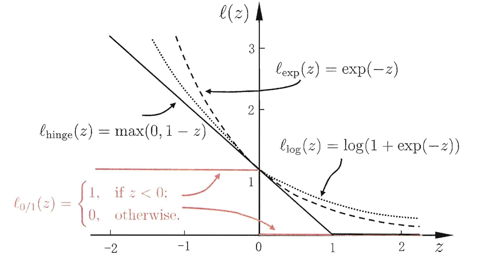
Notice that the Hinge loss is robust to outliers in training data compared to other surrogate loss functions. In the following, we use hinge loss as the surrogate loss.
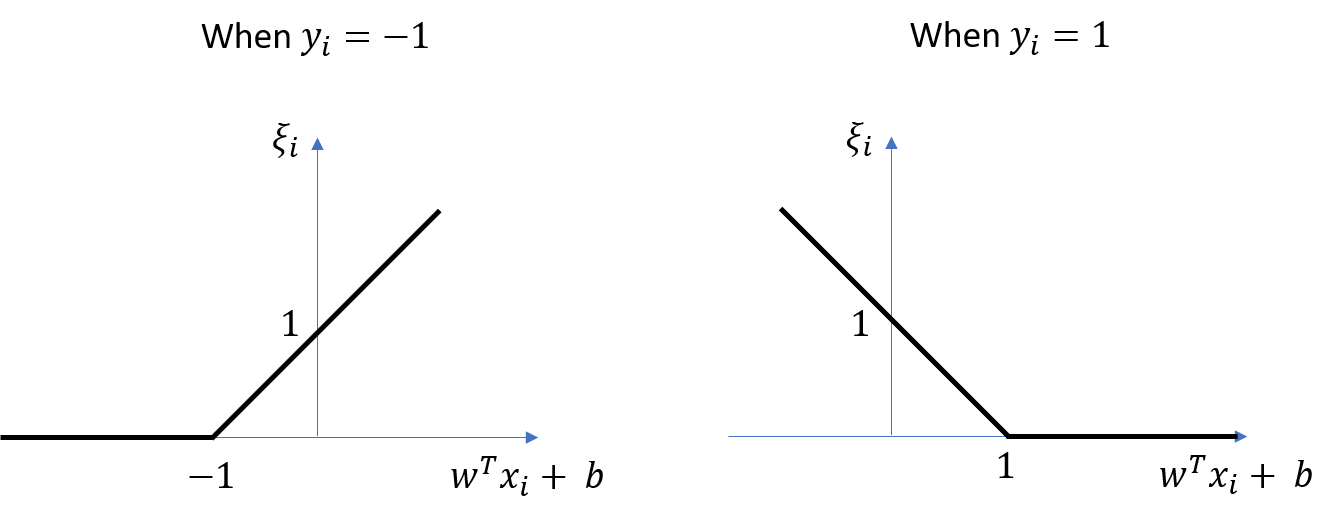
We introduce slack variables \(\xi_i\) to account for violations for linear separability, as
\[\xi_i = \ell_{\text{hinge}}(z_i+1) = \max\left(0, 1 - y_i(w^Tx_i+b)\right).\]The plot of \(\xi_i\) is as shown below.
For a hyperparameter \(C > 0\), the soft margin SVM is then:
\[\begin{equation*} \begin{aligned} & \min_{w,b} \frac{\|w\|}{2} + C \sum_{i=1}^{n} \xi_i,\\ & \text{ subject to } \begin{cases} y_i(w^Tx_i+b) \geq 1-\xi_i, \\ \xi_i\geq0, \end{cases} \ \ \forall i=1,\cdots,n. \end{aligned} \end{equation*}\]The points \(\{(x_i, y_i): y_i(\hat{w}^Tx_i+\hat{b}) \leq 1\}\) are the support vectors.
Let \(\hat{w}, \hat{b}\) be the solution of the optimization, then the seperating hyperplane is
\[\{ x \in \mathbb{R}^p : \hat{w}^T x + \hat{b} = 0 \}\]and the prediction is
\[\hat{y} = \text{sign}(\hat{w}^Tx + \hat{b}).\]Lagrange Duality
Dual Optimization Problem
The Lagrange function of the optimization problem of soft margin SVM is
\[\mathcal{L}(w,b,\xi,\alpha,\mu) = \frac{\|w\|^2}{2} + C \sum_{i=1}^{n} \xi_i + \sum_{i=1}^n \alpha_i [1 - \xi_i - y_i(w^Tx_i + b)] - \sum_{i=1}^n\mu_i\xi_i,\]where \(\alpha_i \geq 0, \mu_i \geq 0\) are the Lagrange multipliers.
Set
\[\mathcal{D}(\alpha,\mu) = \min_{w,b,\xi} \mathcal{L}(w,b,\xi,\alpha,\mu).\]Then the dual optimization problem is
\[\max_{\alpha, \mu: \alpha_i \geq 0, \mu_i \geq 0} \mathcal{D}(\alpha,\mu) = \max_{\alpha, \mu: \alpha_i \geq 0, \mu_i \geq 0} \min_{w,b,\xi} \mathcal{L}(w,b,\xi,\alpha,\mu).\]Take derivative of \(\mathcal{L}(w,b,\xi,\alpha,\mu)\) with respect to \(w,b,\xi_i\) and set equal to \(0\), and we have
\[\begin{aligned} & \frac{\partial \mathcal{L}(w,b,\xi,\alpha,\mu)}{\partial w} = w - \sum_{i=1}^{n} \alpha_i y_i x_i = 0 \implies w = \sum_{i=1}^{n} \alpha_i y_i x_i, \\ & \frac{\partial \mathcal{L}(w,b,\xi,\alpha,\mu)}{\partial b} = - \sum_{i=1}^{n} \alpha_i y_i = 0 \implies \sum_{i=1}^{n} \alpha_i y_i = 0, \\ & \frac{\partial \mathcal{L}(w,b,\xi,\alpha,\mu)}{\partial \xi_i} = C - \alpha_i - \mu_i = 0 \implies \alpha_i + \mu_i = C. \end{aligned}\]Plug these three equations into \(\mathcal{L}(w,b,\xi,\alpha,\mu)\), then the previous dual optimization problem can be rewritten as:
\[\begin{equation*} \begin{aligned} & \max_{\alpha} \mathcal{D}(\alpha) = \sum_{i=1}^n \alpha_i - \frac{1}{2} \sum_{i=1}^n \sum_{i'=1}^n \alpha_i\alpha_{i'}y_iy_{i'}x_i^Tx_{i'}, \\ & \text{ subject to } \begin{cases} \sum_{i=1}^n \alpha_iy_i=0, \\ 0\leq\alpha_i\leq C , \end{cases} \ \ \forall i=1,\cdots,n. \end{aligned} \end{equation*}\]Note that there are inequity constraints in the optimization formulation, thus we have the KKT condtions:
\[\begin{cases} \alpha_i \geq 0, \\ \mu_i \geq 0, \\ y_i(w^Tx_i+b) - 1 + \xi_i \geq 0, \\ \alpha_i[y_i(w^Tx_i+b) - 1 + \xi_i] = 0, \\ \xi_i \geq 0, \\ \mu_i\xi_i = 0. \end{cases}\]Compared to the orginal optimization problem, the constraints in the dual problem are easier to do optimization, and also we can apply kernel trick in the dual problem.
SMO Algorithm
We use the SMO (sequential minimal optimization) algorithm to solve the dual optimization problem. The basic idea is that, if all variables satisfy the KKT conditions, these variables are the solution, because the KKT conditions are necesary and suffcient conditions for the dual optimization problem.
It simply does the following:
Repeat till convergence {
-
Select some pair \(α_i\) and \(α_{i'}\) to update next (using a heuristic that tries to pick the two that will allow us to make the biggest progress towards the global maximum).
-
Reoptimize \(\mathcal{D}(\alpha)\) with respect to \(α_i\) and \(α_{i'}\) , while holding all the other \(α_{i''}\)’s \((i'' \neq i, i')\) fixed. }
The solution of the dual optimization problem is
\[\hat{\alpha} = (\hat{\alpha}_1, \hat{\alpha}_2, \cdots, \hat{\alpha}_n) = \arg\max_{\alpha} \mathcal{D}(\alpha),\]Solution
After getting the solution \(\hat{\alpha}\), we have the weight
\[\hat{w} = \sum_{i=1}^n \hat{\alpha}_{i} y_{i}x_{i}.\]The support vectors are the data points \((x_i,y_i)\) that have the indexes in the set:
\[I^* = \{ i^*: \hat{\alpha}_{i^*} \neq 0 \} = \{ i^*: 0 < \hat{\alpha}_{i^*} \leq C \}.\]Then we compute the intercept \(\hat{b}\) by any support vector \((x_{i^*},y_{i^*})\):
\[\hat{b} = y_{i^*} - \hat{w}^Tx_{i^*} = y_{i^*} - \sum_{i=1}^n \hat{\alpha}_{i} y_{i}x_{i}^T x_{i^*}.\]In practice, it is more robust to calculate the average of \(\hat{b}\) by all (or some) support vectors:
\[\hat{b} = \frac{1}{\mid I^* \mid} \sum_{i^* \in I^*} \left( y_{i^*} - \hat{w}^Tx_{i^*} \right) = \frac{1}{\mid I^* \mid} \sum_{i^* \in I^*} \left( y_{i^*} - \sum_{i=1}^n \hat{\alpha}_{i} y_{i}x_{i}^T x_{i^*} \right).\]The separating hyperplane is
\[\left\{ x\in\mathbb{R}^p: \hat{w}^T{x} + \hat{b} = 0 \right\} = \left\{ x\in\mathbb{R}^p: \sum_{i=1}^n \hat{\alpha}_{i} y_{i}x_{i}^T x + \frac{1}{\mid I^* \mid} \sum_{i^* \in I^*} \left( y_{i^*} - \sum_{i=1}^n \hat{\alpha}_{i} y_{i}x_{i}^T x_{i^*} \right) = 0 \right\}.\]The output of the classifier is
\[\hat{y} = \text{sign} \left( \hat{w}^Tx + \hat{b} \right).\]Support Vectors
For a sample \((x_i,y_i)\), there are five different situations:
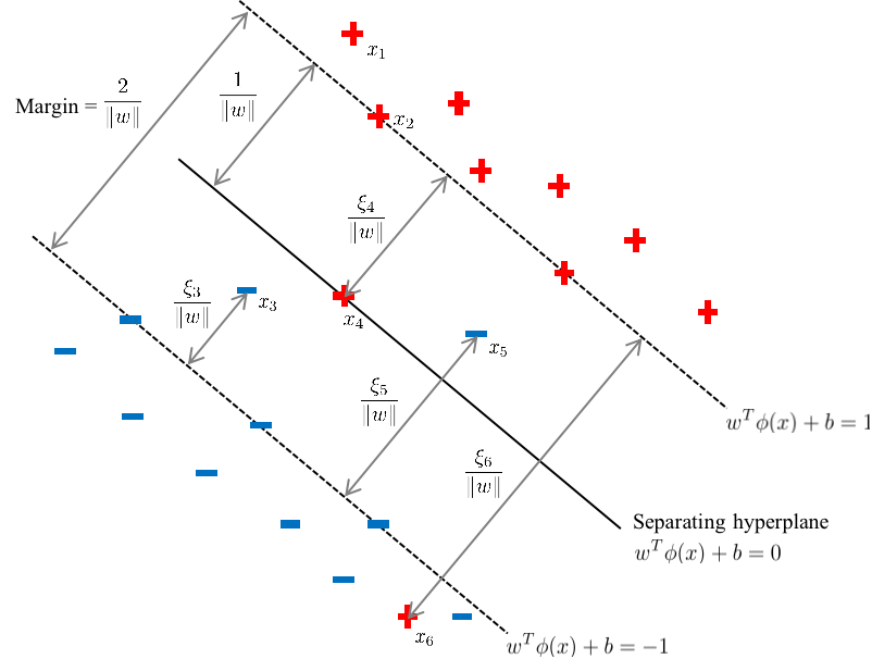
If \(\alpha_i=0\), then \(\mu_i=C,\xi_i=0\). The sample (e.g. \(x_1\) in the plot below) does not affect the estimation of the hyperplane \(\left\{ x\in\mathbb{R}^p: \hat{w}^T{x} + \hat{b} = 0 \right\}\), and this sample is not a support vector.
Otherwise, when \(0 < \alpha_i \leq C\), the sample is a support vector.
If \(0<\alpha_i<C\), then \(\mu_i=C-\alpha_i,\xi_i=0\). This sample (e.g. \(x_2\) in the plot below) is correctly classified, and on the hyperplane \(H_1\) if \(y_i=1\) or \(H_2\) if \(y_i=-1\).
When \(\alpha_i=C\), it follows that \(\mu_i=0\), and \(\frac{\xi_i}{\|w\|}>0\) is the distance between the sample and the hyperplane \(H_1\) if \(y_i=1\) or \(H_2\) if \(y_i=-1\).
If \(\alpha_i=C\) and \(0<\xi_i<1\), then \(\mu_i=0\). This sample (e.g. \(x_3\) in the plot below) is correctly classified.
If \(\alpha_i=C\) and \(\xi_i=1\), then \(\mu_i=0\). This sample (e.g. \(x_4\) in the plot below) is on the separating hyperplane.
If \(\alpha_i=C\) and \(\xi_i>1\), then \(\mu_i=0\). This sample (e.g. \(x_5,x_6\) in the plot below) is incorrectly classified and beyond the separating hyperplane.
These five situations are summarized as below:
| \(\alpha_i\) | \(\mu_i\) | \(\xi_i\) | Is correctly classificed? | Is a support vector? | Is on the hyperplane? |
|---|---|---|---|---|---|
| \(0\) | \(C\) | \(0\) | Yes | No | No |
| \(0<\alpha_i<C\) | \(C-\alpha_i\) | \(0\) | Yes | Yes | On \(H_1\) if \(y_i=1\) or \(H_2\) if \(y_i=-1\). |
| \(C\) | \(0\) | \(0<\xi_i<1\) | Yes | Yes | No |
| \(C\) | \(0\) | \(1\) | / | Yes | On the separating hyperplane. |
| \(C\) | \(0\) | \(\xi_i>1\) | No | Yes | In case \(\xi_i=2\), on \(H_2\) if \(y_i=1\) or \(H_1\) if \(y_i=-1\). Otherwise no. |
Kernel SVM
Mapping to a Higher Feature Space
If the data is not linearly separable and it has finite features, mapping to a higher dimensional feature space makes it linearly separable.
As an example shown below, the left plot shows that the data is not linearly separable in original feature space, while the right plot shows that the data is linearly separable in a higher dimensional feature space.
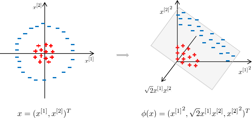
Denote \(\phi:\mathbb{R}^p \to \mathbb{R}^\tilde{p}\) as a mapping function and \(\phi(x)\) as the higher dimensional feature vector after mapping \(x\) to a higher dimensional feature space:
\[x \in \mathbb{R}^p \to \phi(x) \in \mathbb{R}^\tilde{p}.\]Then the two hyperplanes will be
\[\{x \in \mathbb{R}^p : w^T \phi(x) + b = \pm 1\}.\]The soft margin SVM is then:
\[\begin{equation*} \begin{aligned} & \min_{w,b} \frac{\|w\|}{2} + C \sum_{i=1}^{n} \xi_i, \\ & \text{ subject to } \begin{cases} y_i(w^T \phi(x_i)+b) \geq 1-\xi_i, \\ \xi_i \geq 0, \end{cases} \ \ \forall i=1,\cdots,n. \end{aligned} \end{equation*}\]The dual optimization problem:
\[\begin{equation*}\begin{aligned}& \min_{\alpha} \mathcal{D}(\alpha) = \sum_{i=1}^n \alpha_i - \frac{1}{2} \sum_{i=1}^n \sum_{i'=1}^n \alpha_i\alpha_{i'}y_iy_{i'} \phi(x_i)^T \phi(x_{i'}), \\ & \text{ subject to } \begin{cases} \sum_{i=1}^n \alpha_iy_i=0, \\ 0\leq\alpha_i\leq C , \end{cases} \ \ \forall i=1,\cdots,n. \end{aligned} \end{equation*}\]Kernel Trick
Since the feature vector \(\phi(x)\) may have a very high dimension \(\tilde{p}\), the computation of the inner product \(\phi(x_i)^T \phi(x_{i'})\) is \(O(\tilde{p})\) and is extremely expensive. To deal with that, we use the kernel trick.
A kernel function is defined as
\[\mathcal{K}(x_i, x_{i'}) = \phi(x_i)^T \phi(x_{i'}).\]With the kernel function, we can compute the inner product \(\phi(x_i)^T \phi(x_{i'})\) by using \(x_i, x_{i'}\) that are in the original space, and the computation of \(\mathcal{K}(x_i, x_{i'})\) is \(O(p)\). By using kernel function, the computation is reduced from \(O(\tilde{p})\) to \(O(p)\). That means computing \(\mathcal{K}(x_i, x_{i'})\) is much cheaper than computing \(\phi(x_i)^T \phi(x_{i'})\) directly.
Applying kernel trick on SVM, the dual optimization problem can be rewritten as
\[\begin{equation*}\begin{aligned}& \min_{\alpha} \mathcal{D}(\alpha) = \sum_{i=1}^n \alpha_i - \frac{1}{2} \sum_{i=1}^n \sum_{i'=1}^n \alpha_i\alpha_{i'}y_iy_{i'} \mathcal{K}(x_i, x_{i'}), \\ & \text{ subject to } \begin{cases} \sum_{i=1}^n \alpha_iy_i=0, \\ 0\leq\alpha_i\leq C , \end{cases} \ \ \forall i=1,\cdots,n. \end{aligned} \end{equation*}\]The separating hyperplane is
\[\left\{ x\in\mathbb{R}^p: \hat{w}^T{x} + \hat{b} = 0 \right\} = \left\{ x\in\mathbb{R}^p: \sum_{i=1}^n \hat{\alpha}_{i} y_{i}\mathcal{K}(x_i, x) + \frac{1}{\mid I^* \mid} \sum_{i^* \in I^*} \left( y_{i^*} - \sum_{i=1}^n \hat{\alpha}_{i} y_{i}\mathcal{K}(x_i, x_{i^*}) \right) = 0 \right\}.\]The kernel matrix is defined as
\[\mathbf{K} = \begin{pmatrix} \mathcal{K}(x_1, x_1) & \mathcal{K}(x_1, x_2) & \cdots & \mathcal{K}(x_1, x_{n}) \\ \mathcal{K}(x_2, x_1) & \mathcal{K}(x_2, x_2) & \cdots & \mathcal{K}(x_2, x_{n}) \\ \vdots & \vdots & \ddots & \vdots \\ \mathcal{K}(x_n, x_1) & \mathcal{K}(x_n, x_2) & \cdots & \mathcal{K}(x_n, x_{n}) \end{pmatrix}.\]Kernel matrix is always positive semi-definite. Actually a function \(\mathcal{K}(x_i, x_{i'})\) can be used as a kernel function if and only if it is symmetric and the corresponding kernel matrix is positive semi-definite. The function is symmetric means that \(\mathcal{K}(x_i, x_{i'}) = \mathcal{K}(x_{i'}, x_i)\) for all \(i,i'\).
Some commonly used kernel functions:
| Name | Formula | Hyperparameter |
|---|---|---|
| Linear | \(\mathcal{K}(x_i, x_{i'})=x_i^Tx_{i'}\) | |
| Polynomial | \(\mathcal{K}(x_i, x_{i'})=(x_i^Tx_{i'})^d\) | polynomal degree \(d > 1\) |
| RBF (or Gaussian) | \(\mathcal{K}(x_i, x_{i'})=\exp (-| x_i - x_{i'} |/2\sigma^2)\) | width \(\sigma>0\) |
| Laplace | \(\mathcal{K}(x_i, x_{i'})=\exp (-| x_i - x_{i'}|/\sigma)\) | \(\sigma>0\) |
| Sigmoid | \(\mathcal{K}(x_i, x_{i'})=\text{tanh}(\beta x_i^Tx_{i'} + \theta)\) | \(\beta>0, \theta<0\) |
How to choose?
- If the number of features is large, and sample size is small, the data is usually linearly separable, then use linear kernel or logistic regression.
- If the number of features is small, and sample size is normal, then use RBF kernel.
- If the number of features is small, and sample size is large, then add some features and it becomes the first case.
Note that SVMs with linear kernel are linear classifiers, and SVMs with other kernels are non-linear classifiers.
SVR
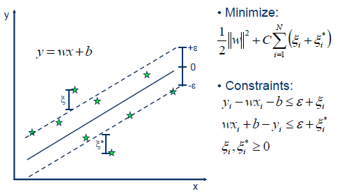
In SVR (support vector regression), we tolerate an error \(\epsilon\) between \(w^Tx+b\) and \(y\), which means the error will not be considered if it is within $-\epsilon$ and \(\epsilon\). Note that \(\epsilon\) is a hyperparameter that we should set before training the model.
Tips
The optimum of SVM must be the global optimum, since it is a convex optimization problem.
SVM is good for small sample size, compared to other machine learning methods, since we only need a few support vectors to determine the hyperplanes. SVM is also suitable for non-linear and high dimensional problems.
SVM is not very sensitive to imbalanced dataset problem. The loss is composed by margin and support vectors, not by all data, thus SVM works well if the support vectors are balanced, and the balanced original dataset is not that necessary.
References:
Lecture notes from my professor Min Xu.
李航. 第7章 支持向量机. 统计学习方法. 清华大学出版社, 2012.
周志华. 机器学习. 清华大学出版社, 2016.
张皓. 从零推导支持向量机(SVM).