Optimization

Given a neural network, the goal of the training procedure is to learn parameters $W^{[l]}$ and $b^{[l]}$ for each layer $l$ that minimize the loss function plus regularization term.

We first assume there are $n^{[l-1]}$ hidden units in the hidden layer $l-1$ and $n^{[l]}$ units in the layer $l$. Denote the output of the layer \(l-1\) (it is also the input of the layer \(l\)) as $a^{[l-1]} \in \mathbb{R}^{n^{[l-1]}}$. In the layer \(l\), denote the weight matrix as $W^{[l]} \in \mathbb{R}^{n^{[l]}\times n^{[l-1]}}$, bias vector as $b^{[l]}\in\mathbb{R}^{n^{[l]}}$, activation function as \(\sigma^{[l]}(\cdot)\), then the output of the layer \(l\) is

\[a^{[l]} = \sigma^{[l]}(W^{[l]} a^{[l-1]} + b^{[l]}) \in \mathbb{R}^{n^{[l]}}.\]

Loss Function

The observations for target variable are \(y=(y_1,y_2,\cdots,y_n)^T\in\mathbb{R}^n\), and the corresponding predictions are \(\hat{y}=(\hat{y}_1, \hat{y}_2, \cdots, \hat{y}_n)^T \in \mathbb{R}^n\).

For regression problems, the L2 loss is most commonly used:

\[L(\hat{y}_i, y_i) = (y_i - \hat{y}_i)^2, \text{ or } L(\hat{y}, y) = \| \hat{y} - y \|_2^2.\]

For $K$-class classification problems, we usually use cross-entropy loss function:

\[L(\hat{p}_i, y_i) = -\sum_{k=1}^{K} \mathbf{1}(y_i \text{ in class } k)\log(\hat{p}_{ik}),\]

where \(\hat{p}_{ik}\) is the estimated probability of $y_i$ belongs to class $k$, and \(\mathbf{1}(\cdot)\) is the indicator function. The estimated probabilities \(\hat{p}_{ik}\) is usually calculated by softmax function: \(\hat{p}_{ik} = \frac{e^{z_{ik}}}{\sum _{k=1}^{K}e^{z_{ik}}}\).

For binary classification, the cross-entropy loss is

\[L(\hat{p}_i, y_i) = -y_i\log(\hat{p}_i) - (1-y_i)\log(1-\hat{p}_i),\]

where $y_i\in{0,1}$, $\hat{p}_i$ is the estimated probability of $y_i=1$.

Initialization

If all weights are initialized to the same value, the activations of neurons in each layer are same, and the gradients of weights in each layer are same, it follows that the network has the same effectiveness as a network that has only single neuron in each layer. In a special case that all weights are initialized to \(0\) and we use the activation function that \(\sigma(0)=0\) (such as Tanh, ReLU), then all activations and gradients are \(0\), and the weights cannot be updated through gradient descent. Thus, the weights in same layer should be initialized differently (usually randomly) to break symmetry during training.

If the weights in a network start too small/large, then the backpropagated gradient signal shrinks/grows as it passes through and it may lead to vanishing/exploding gradients, and that can result in divergence/slow-down in the training of the network.

The appropriate initialization that follows the rules below guarantees no exploding/vanishing (either forward or backward) signal.

1. The mean (expectation) of the activations should be same and be zero. i.e. \(E(a^{[l-1]}) = E(a^{[l]})=0\);
2. The variance of the activations should stay the same across every layer. i.e. \(\text{Var}(a^{[l-1]}) = \text{Var}(a^{[l]})\).

Xavier Initialization

Xavier initialization was introduced by Glorot Xavier, and it works for activation functions like sigmoid, tanh and linear etc..

That is, for every layer $l$, we initialize

\[W^{[l]} \sim N\left(0,\frac{1}{n^{[l-1]}}\right) \text{ or } N\left(0,\frac{2}{n^{[l-1]} + n^{[l]}}\right), \ b^{[l]}=0.\]

We first derive the Xavier initialization through the forward propagation. Now the purpose of the initialization is to avoid the vanishing or exploding of the forward propagated signal.

Based on some assumptions (assume the activation function is tanh. etc.), we can show that

\[\text{Var}(a^{[l]}) = n^{[l-1]} \text{Var}(W^{[l]}) \cdot \text{Var}(a^{[l-1]}).\]

It follows that setting \(\text{Var}(W^{[l]}) = 1/n^{[l-1]}\) leads to \(\text{Var}(a^{[l-1]}) = \text{Var}(a^{[l]})\).

At every layer, we can link this layer’s variance to the input layer’s variance:

\[\begin{align} \text{Var}(a^{[l]}) &= n^{[l-1]} \text{Var}(W^{[l]}) \cdot \text{Var}(a^{[l-1]}) \\ &= n^{[l-1]} \text{Var}(W^{[l]}) \cdot n^{[l-2]} \text{Var}(W^{[l-1]}) \cdot \text{Var}(a^{[l-2]}) \\ &= \cdots \\ &= \left[ \prod_{s=1}^l n^{[s-1]} \text{Var}(W^{[s]}) \right] \cdot \text{Var}(x). \end{align}\]

Then we have the following three cases:

\[\begin{align} &\text{For all } s=1,\cdots,l, \\ &n^{[s-1]} \text{Var}(W^{[s]}) \begin{cases} <1 \implies \text{Var}(a^{[l]}) \ll \text{Var}(x); \\ =1 \implies \text{Var}(a^{[l]}) = \text{Var}(x); \\ >1 \implies \text{Var}(a^{[l]}) \gg \text{Var}(x). \\ \end{cases} \end{align}\]

Since the mean is zero (i.e. \(E(a^{[l]})=0\)), low variance (i.e. \(\text{Var}(a^{[l]})\) is small) means that the activations \(a^{[l]}\) would be very close to zero (forward signal vanishing), and high variance means that the activations would be very large in absolute value (forward signal exploding).

Throughout the justification, we worked on activations computed during the forward propagation, and we conclude that, to avoid the vanishing or exploding of the forward propagated signal, we initialize

\[\text{Var}(W^{[l]}) = \frac{1}{n^{[l-1]}}.\]

The same result can be derived for the backpropagated gradients. Doing so, you will see that in order to avoid the vanishing or exploding gradient problem, we should initialize

\[\text{Var}(W^{[l]}) = \frac{1}{n^{[l]}}.\]

As a compromise, we can roughly took the harmonic mean of the two:

\[\text{Var}(W^{[l]}) = \frac{2}{n^{[l-1]} + n^{[l]}}.\]

He Initialization

He initialization was introduced by Kaiming He, and it works for activation functions like ReLU and leaky ReLU etc..

That is, for every layer $l$, we initialize

\[W^{[l]} \sim N\left(0,\frac{2}{n^{[l-1]}}\right), \ b^{[l]}=0.\]

For activation functions like ReLU and leaky ReLU etc., this initialization avoid the vanishing or exploding of both the forward propagated signal and backpropagated gradients.

Backpropagation

We usually use gradient descent to optimize the objective function $\text{Obj}(w)$. For weight, we have

\[w_t = w_{t-1} - \eta \frac{\partial \text{Obj}(w_{t-1})}{\partial w_{t-1}},\]

where $\eta$ is the step-size (learning rate).

The solution to computing the gradient is an algorithm called error backpropagation, which use the chain rules in calculus. (Note: the regularization term is not considered in the pictures below.)

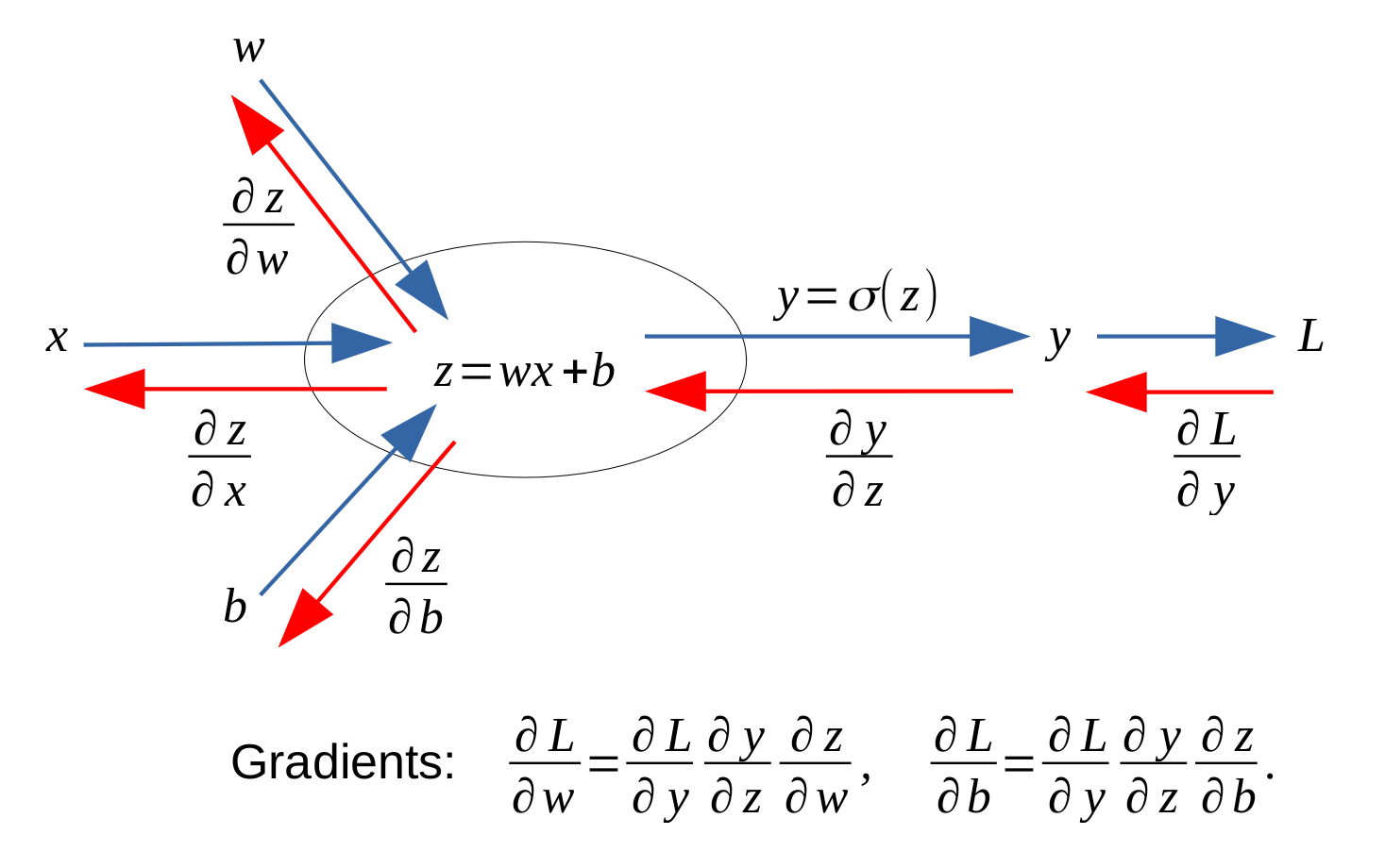
Here let’s take an example. Say there is a feed forward neural network for regression, as shown in the picture below.

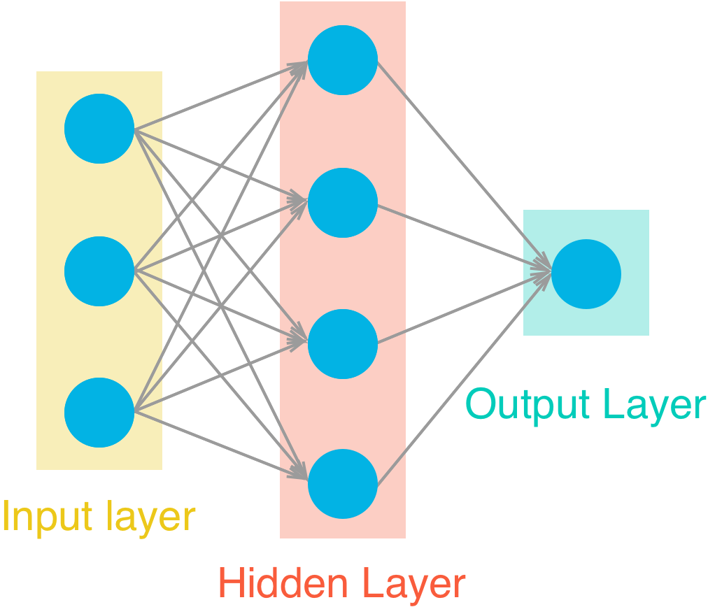
Suppose the activation function \(\sigma(\cdot)\) for hidden layer is sigmoid, and the activation function for output layer is identity function. Denote the input vector as \(x\in\mathbb{R}^{p}\), the target as \(y\in\mathbb{R}\), the output scalar as \(\hat{y}\in\mathbb{R}\), the weights of hidden layer as $W\in\mathbb{R}^{p \times q}$, the weights of output layer as \(V\in\mathbb{R}^{q}\), the loss function as \(L(\hat{y},y)=(\hat{y}-y)^2\). This network can be expressed mathematically as

\[\hat{y} = \sigma(x^TW) \cdot V,\]

where \(x\) is the input of the hidden layer, \(\sigma(x^TW)\) is the output of the hidden layer and is also the input of the output layer, and \(\hat{y}\) is the output of the output layer.

Denote \(w_r\in\mathbb{R}^p\) as the \(r\)-th column vector of \(W\), \(v_r\in\mathbb{R}\) as the $r$-th entry of \(V\), and \(\mathbf{1}\) as an all ones vector. We have \(W = (w_1,w_2,\cdots,w_q)\) and \(V=(v_1,v_2,\cdots,v_q)^T\), then the network can be expressed in summation form as

\[\hat{y} = \sigma(x^TW) \cdot V = \Big( \sigma(x^Tw_1), \cdots, \sigma(x^Tw_q) \Big) \cdot V = \sum_{r=1}^q \sigma(x^Tw_r) v_r.\]

Now let’s compute the gradients for \(v_r\) and \(w_r\):

\[\begin{align} & \frac{\partial L(\hat{y},y)}{\partial v_r} = \frac{\partial L(\hat{y},y)}{\partial \hat{y}} \frac{\partial \hat{y}}{\partial v_r} = 2(\hat{y}-y) \cdot \sigma(w_r^Tx), \\ & \frac{\partial L(\hat{y},y)}{\partial w_r} = \frac{\partial L(\hat{y},y)}{\partial \hat{y}} \frac{\partial \hat{y}}{\partial \sigma(x^Tw_r)} \frac{\partial \sigma(x^Tw_r)}{x^Tw_r} \frac{\partial x^Tw_r}{w_r} = 2(\hat{y}-y) v_r \cdot \sigma(x^Tw_r) [1 - \sigma(x^Tw_r)] \cdot x. \end{align}\]

Or directly the gradients for \(V\) and \(W\):

\[\begin{align} & \frac{\partial L(\hat{y},y)}{\partial V} = \frac{\partial L(\hat{y},y)}{\partial \hat{y}} \frac{\partial \hat{y}}{\partial V} = 2(\hat{y}-y) \cdot \sigma(W^Tx), \\ & \frac{\partial L(\hat{y},y)}{\partial W} = \frac{\partial L(\hat{y},y)}{\partial \hat{y}} \frac{\partial \hat{y}}{\partial \sigma(x^TW)} \frac{\partial \sigma(x^TW)}{x^TW} \frac{\partial x^TW}{W} = 2(\hat{y}-y) x \cdot \big[ V^T \odot \sigma(x^TW) \odot [\mathbf{1} - \sigma(x^TW)] \big]. \end{align}\]

Gradient Descent with Momentum

The basic idea of momentum is to compute an moving average of the gradients, and use that average gradient to update the parameters.

At the \(t\)-th step of gradient update of weights, we have \(w_t = w_{t-1} - \eta v_{w_{t}}\). In standard gradient descent (GD), we set \(v_{w_{t}}\) as \(\frac{\partial\text{Obj}(w_{t-1})}{\partial w_{t-1}}\). But in the gradient descent (GD) with momentum, we set \(v_{w_{t}} = \beta v_{w_{t-1}} + (1-\beta) \cdot \frac{\partial\text{Obj}(w_{t-1})}{\partial w_{t-1}}.\)

The hyperparameter \(\beta\) is usually set to \(0.9\) or a similar value.

In the GD with momentum, if the history gradients \(\frac{\partial\text{Obj}(w_{t'})}{\partial w_{t'}^{(j)}}\), (\(t'=t-1,t-2,\cdots\)) in dimension \(j\) point in the same direction, then the parameter updating amplitude \(\mid v_{w_t^{(j)}} \mid\) is increased through the moving average, compared to the size of the current gradient \(\mid\frac{\partial\text{Obj}(w_{t-1}^{(j)})}{\partial w_{t-1}^{(j)}}\mid\) in standard GD. Otherwise, if the history gradients change directions, the parameter updating amplitude is decreased through the moving average. As a result, GD with momentum accelerates convergence and reduces oscillation.

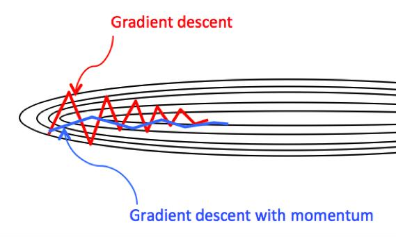
As shown in the plot above, suppose the parameter in horizontal direction is \(w^{(1)}\) and that in vertical direction is \(w^{(2)}\). The updating amplitude \(\mid v_{w_t^{(1)}} \mid\) is increased compared to the size of the current gradient \(\mid\frac{\partial\text{Obj}(w_{t-1}^{(1)})}{\partial w_{t-1}^{(1)}}\mid\), thus the GD with momentum accelerates the convergence of \(w^{(1)}\). On the other hand, the updating amplitude \(\mid v_{w_t^{(2)}} \mid\) is decreased compared to the size of the current gradient \(\mid\frac{\partial\text{Obj}(w_{t-1}^{(2)})}{\partial w_{t-1}^{(2)}}\mid\), thus the GD with momentum reduces the oscillation of \(w^{(2)}\).

Other Tips

Batch Gradient Descent (BGD) is usually computationally expensive, thus we use Stochastic Gradient Descent (SGD) or Mini-Batch Gradient Descent (MBGD).

In SGD, at every gradient updating step, we take only one example to calculate the gradient, and update the parameters.

In MBGD, we use a batch of a fixed number of training examples which is less than the actual dataset and call it a mini-batch. We first create the mini-batches of fixed size, at every epoch, we iterate over every mini-batches, and calculate the mean gradient of the mini-batch, and update the parameters.

However, SGD and MBGD are more sensitive to learning rate and initialization. A large learning rate or an improper initialization may lead to vanishing gradient or exploding gradient.

References:

Goodfellow, Ian, Yoshua Bengio, and Aaron Courville. Deep learning. MIT press, 2016.

Glorot, Xavier, and Yoshua Bengio. “Understanding the difficulty of training deep feedforward neural networks.” Proceedings of the thirteenth international conference on artificial intelligence and statistics. 2010.

He, Kaiming, et al. “Delving deep into rectifiers: Surpassing human-level performance on imagenet classification.” Proceedings of the IEEE international conference on computer vision. 2015.

Katanforoosh & Kunin. “Initializing neural networks”. DeepLearning.AI. 2019.

CS231n Convolutional Neural Networks for Visual Recognition.

Ng, Andrew. “Gradient descent with momentum”. DeepLearning.AI.