General Tree

A tree is a collection of nodes. The collection can be empty; otherwise, a tree consists of

• a distinguished node called the root $r$;
• and zero or more nonempty (sub)trees, each of whose roots are connected by a directed edge from $r$.

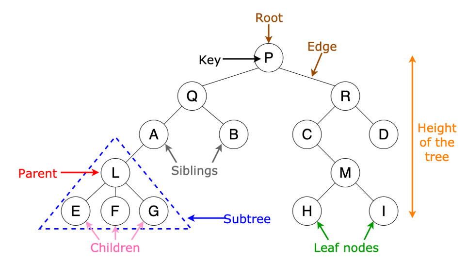
We define the depth of a node as the length of the unique path from the root to the node, and the height of a node as the longest path from the node to a leaf. In the plot above,

Binary Tree

A binary tree is a tree data structure in which a node can have at most two child nodes.

# definition for a binary tree node.
class TreeNode:
    def __init__(self, x):
        self.val = x
        self.left = None
        self.right = None

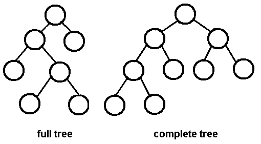
A full binary tree is a binary tree in which each node has exactly zero or two children. A complete binary tree is a binary tree, which is completely filled, with the possible exception of the bottom level, which is filled from left to right.

Tree Traversals

• Preorder: node -> left -> right;
• Inorder: left -> node -> right;
• Postorder: left -> right -> node.

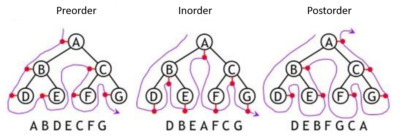
Postorder traversal can compute the heights of the nodes, while preorder tarversal can compute the depths of the nodes.

# traverse a binary tree recursively.
def traverseTreeRecursively(self, root: TreeNode) -> tuple:
    preorder, inorder, postorder = list(), list(), list()
    def recursion(node: TreeNode):
        if node:
            preorder.append(node.val) # preorder traversal
            recursion(node.left)
            inorder.append(node.val) # inorder traversal
            recursion(node.right)
            postorder.append(node.val) # postorder traversal

        recursion(root)
        return preorder, inorder, postorder

Binary Search Tree

A binary search tree (BST) is a binary tree, in which the value (or key) of the left child of a given node should be less than or equal to the parent value and the value of the right child should be greater than or equal to the parent value. That is, left.val <= node.val <= right.val.

Inorder traversal of BST gives nodes in non-decreasing order, and thus BST can be used to implement simple sorting algorithms.

Given a tree with $N$ nodes, the average time complexity of search in a binary tree is $O(N)$, but it is $O(\log_2N)$ for BST, since $\log_2N$ is the average depth of a binary tree (or BST). For the same reason, the average time complexity of insertion and deletion in a BST is also $O(\log_2N)$.

However, in the worst case, BST can have $O(N)$ height, when the skewed tree resembles a linked list. As shown below,

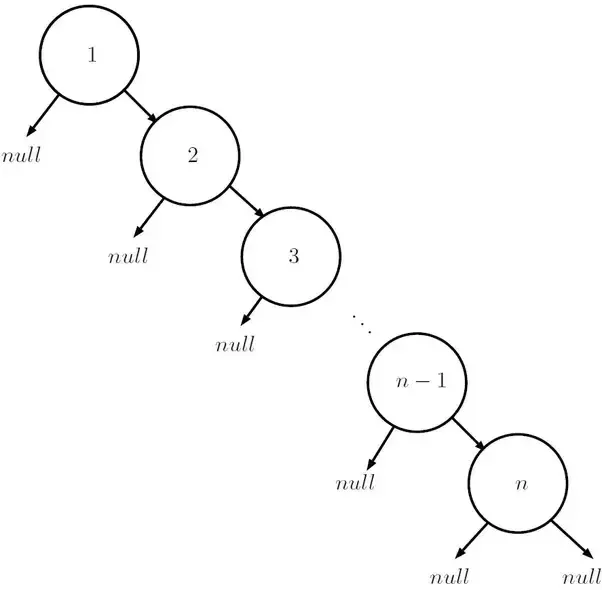
In this worst case, the time complexity of search, insertion and deletion in a BST is $O(N)$.

AVL Tree

An AVL tree is a self-balancing BST, in which each node stores a value called a balance factor which is the difference in height between its left subtree and right subtree and all the nodes must have a balance factor of $-1$, $0$ or $1$.

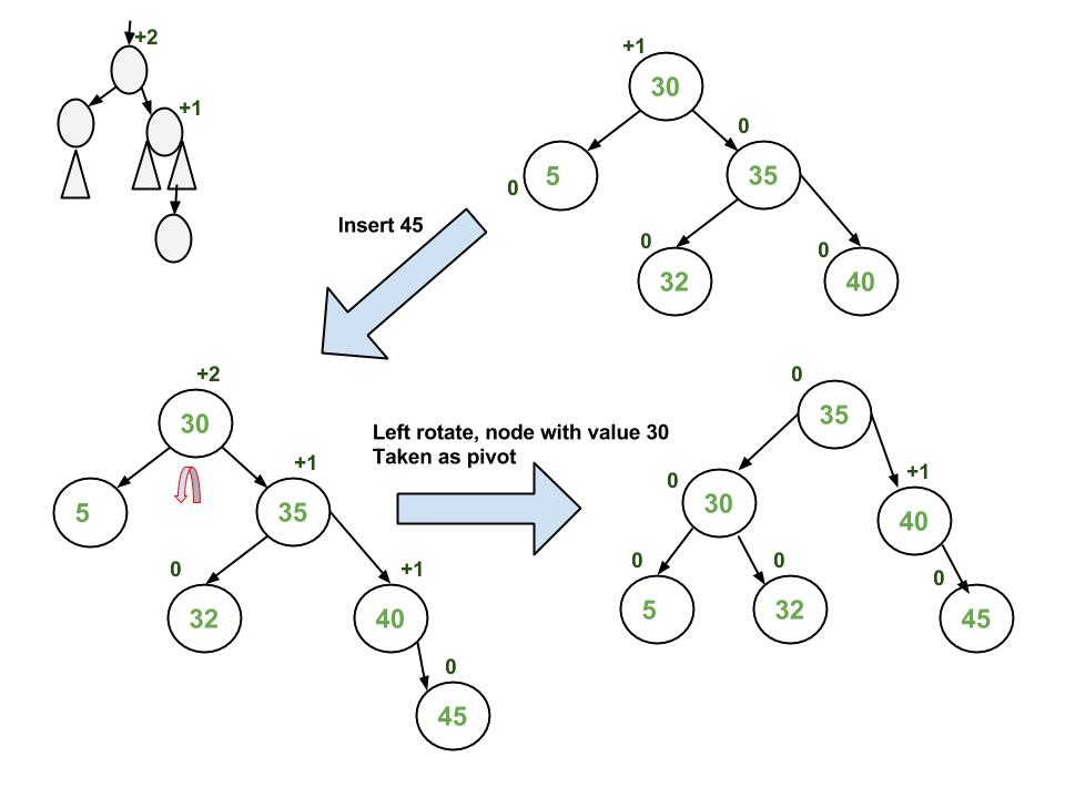
The height of an AVL tree is always $O(\log_2 N)$. Thus, either in the average or worst case, the time complexity of search, insertion and deletion in a AVL tree is $O(\log_2N)$.

Red Black Tree

A red-black tree is a self-balancing BST in which every node follows following rules:

• Every node is either red or black;

• The root is black;

• Every leaf (denoted as NIL) is black;

• Every path from a node (including root) to any of its descendant leaf node has the same number of black nodes.

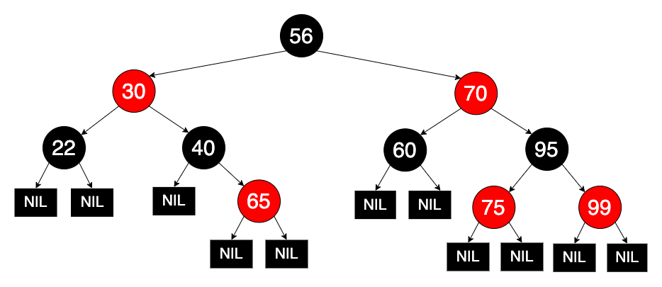
Similar to AVL trees, the height of a red-black tree is always $O(\log_2 N)$. Thus, either in the average or worst case, the time complexity of search, insertion and deletion in a red-black tree is $O(\log_2N)$.

AVL Tree v.s. Red Black Tree

AVL tree: more balanced; Red-black tree: less rotations.

The AVL tree and other self-balancing search trees like Red Black are useful to get all basic operations done in $O(\log_2 n)$ time. The AVL trees are more balanced compared to red-black trees, but they may cause more rotations during insertion and deletion. So if your application involves many frequent insertions and deletions, then red-black trees should be preferred. And if the insertions and deletions are less frequent and search is the more frequent operation, then AVL tree should be preferred.

Splay Tree

A splay tree is a self-balancing BST in which the most recently accessed node is pushed to the root by a series of rotations, and thus it is quick to be accessed again.

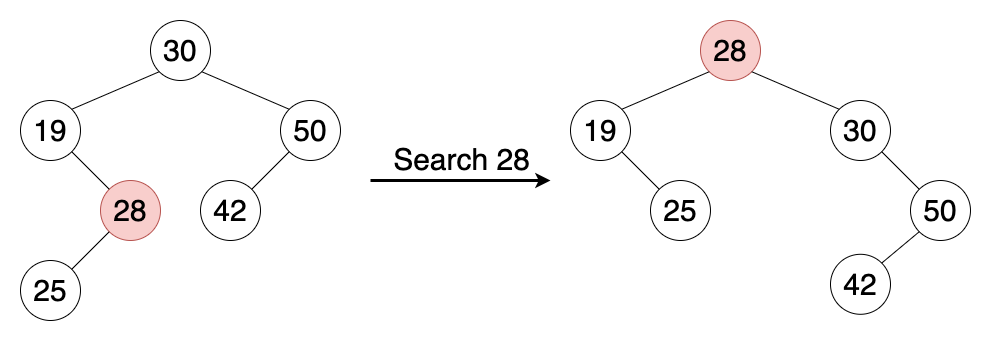
In a splay tree, the frequently accessed nodes will move nearer to the root where they can be accessed more quickly. The worst-case height (though unlikely) is $O(N)$, with the average being $O(\log_2N)$. Having frequently-used nodes near the root is an advantage for many practical applications like locality of reference, and is particularly useful for implementing caches and garbage collection algorithms.

The amortized time complexity of search, insertion and deletion in a splay tree is $O(\log_2N)$. That is, any $S$ consecutive tree operations take at most $O(S \log_2 N)$ time.

B-Tree

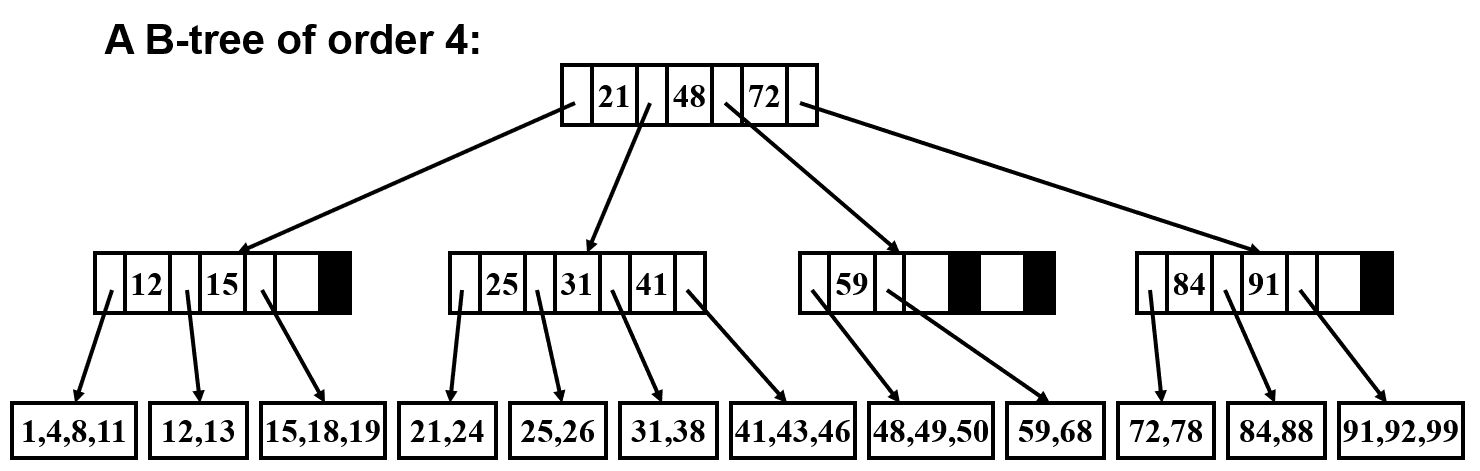
A B-tree is a self-balancing search tree that keeps data in sorted order. A B-tree of order $M$ is a tree which satisfies the following properties:

• All actual data are stored at the leafs;

• The root is either a leaf or has between $2$ and $M$ children;

• Nonleaf nodes (except the root) have between $\frac{M}{2}$ and $M$ children;

• All leaves are at the same depth.

Either in the average or worst case, the time complexity of search, insertion and deletion in a B-tree of order $M$ is $O(\log_MN)$.

Compared with Other Self-Balancing Search Trees

When the data is too huge to fit in main memory and the data is read from disk, the total disk accesses in a B-tree are reduced significantly since the height of the B-tree is low.

In most of the other self-balancing search trees (like AVL and red-black trees), it is assumed that everything is in main memory. To understand the use of B-Trees, we must think of the huge amount of data that cannot fit in main memory. When the number of keys is high, the data is read from disk in the form of blocks. Disk access time is very high compared to the main memory access time.

The main idea of using B-Trees is to reduce the number of disk accesses. Most of the tree operations (search, insert, delete, max, min, etc.) require $O(h)$ disk accesses where $h$ is the height of the tree. B-tree is a fat tree. The height of B-Trees is kept low by putting maximum possible keys in a B-Tree node. Generally, the B-Tree node size is kept equal to the disk block size. Since the height of the B-tree is low so total disk accesses for most of the operations are reduced significantly compared to balanced BST like AVL Tree, red-black Tree, etc..

References:

Allen, W. M. (2007). Data structures and algorithm analysis in C++. Pearson Education India.

https://www.cs.cmu.edu/~adamchik/15-121/lectures/Trees/trees.html.

https://www.geeksforgeeks.org.

https://www.bigocheatsheet.com.

https://towardsdatascience.com/8-useful-tree-data-structures-worth-knowing-8532c7231e8c.