K-Means

The aim of clustering is to divide observations into several non-overlap clusters, such that observations in the same cluster are similar to each other, while observations in different clusters are dissimilar to each other. The clustering problem is an unsupervised learning problem. We are given the training data set \(X = (x_1, x_2, \cdots, x_n)^T \in \mathbb{R}^{n \times p}\), where each observation $x_i \in \mathbb{R}^{p}$ as usual, and we want to group the data into a few cohesive “clusters”.

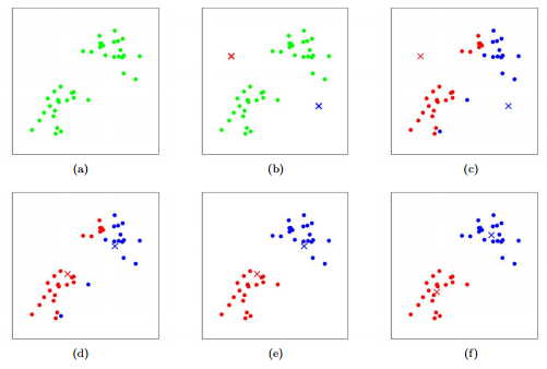
The K-means clustering algorithm is an iterative algorithm. In each step, we assign each data point (observation) to the closest cluster (centroid), then recompute the centroids for the clusters by taking the average of the all data points that belong to each cluster.

Given the hyperparameter \(K\), the objective of K-Means clustering is to minimize total intra-cluster variance, or, the sum of Euclidean distances of samples to their closest cluster: \(D = \sum_{i=1}^n \sum_{k=1}^K \mathbf{1}\{ c_i = k\} \| x_i - \mu_k \|_2^2,\) where \(K\) is the number of clusters, \(c_i\) is the cluster index of \(x_i\), and \(\mu_k\) is the centroid of the cluster \(k\).

Algorithm. K-Means:

[1] Initialize cluster centroids \(\mu_1, \cdots, \mu_K \in \mathbb{R}^p\) randomly.

[2] Repeat until \(\mu_1, \cdots, \mu_K\) do not change:

(a) For every \(i=1, \cdots, n\), set the cluster label for the data point \(i\) as \(c_i := \underset{k}{\text{argmin}} \| x_i - \mu_k \|_2^2\);

(b) For each \(k = 1, \cdots, K\), recompute the the centroid for the cluster \(k\) as \(\mu_k := \frac{\sum_{i=1}^{n} \mathbf{1}\{ c_i = k\} \cdot x_i }{\sum_{i=1}^{n} \mathbf{1}\{ c_i = k\}}\).

Here is a visualization of K-means algorithm:

We can select the hyperparameter \(K\) by the knee point (or elbow point) of the \(D \text{ v.s. } K\) plot, as shown below.

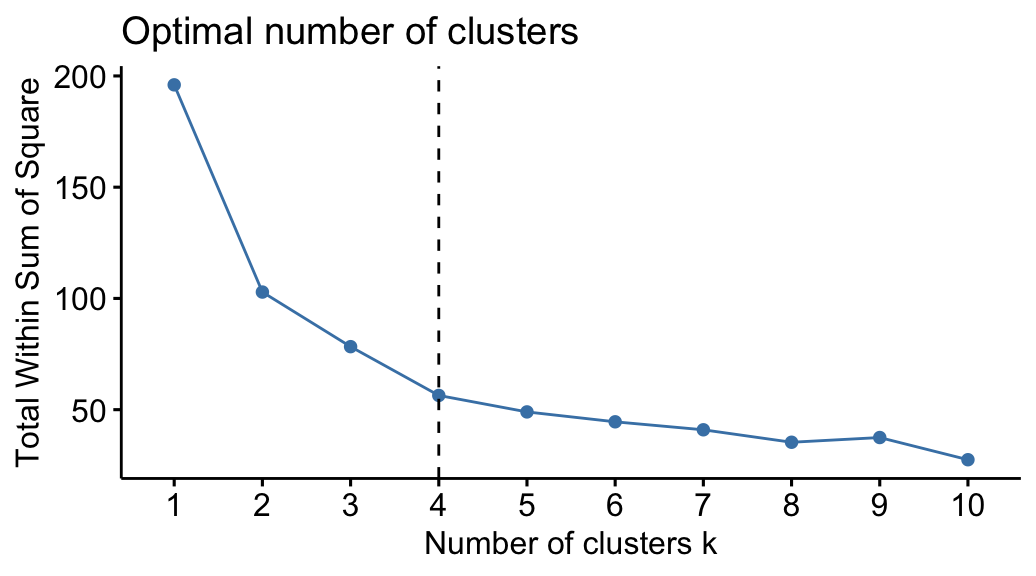
The knee point can also be selected automatically by Kneedle algorithm, or we can identity the suggedted \(K\) by the gap statistic.

K-means algorithm is susceptible to local optima, so we usually reinitialize \(\mu_1, \cdots, \mu_K\) at several different initial parameters.

EM Algorithm

Jensen’s Inequality

Let $f$ be a function whose domain is the set of real numbers (i.e. \(f(x) \in \mathbb{R}\)). Recall that $f$ is a convex function if \(f''(x) ≥ 0\) for all $x ∈ \mathbb{R}$. In the case of $f$ taking vector-valued inputs, this is generalized to the condition that its hessian $H$ is positive semi-definite (\(H ≥ 0\)). We say $f$ is strictly convex if \(f''(x) > 0\) or $H > 0$ for all $x$.

Let $X$ be a random variable, and let $f$ be a convex function, then Jensen’s inequality can then be stated as:

\[E[f(X)] ≥ f(EX).\]

Moreover, if $f$ is strictly convex, then $E[f(X)] = f(EX)$ holds true if and only if $X = E(X)$ with probability $1$ (i.e., if $X$ is a constant).

Note that $f$ is (strictly) concave when $-f$ is (strictly) convex, thus we have \(E[-f(X)] ≥ -f(EX) \implies E[f(X)] \leq f(EX)\) for concave functions $f$.

The figure below is an interpretation of the theorem.

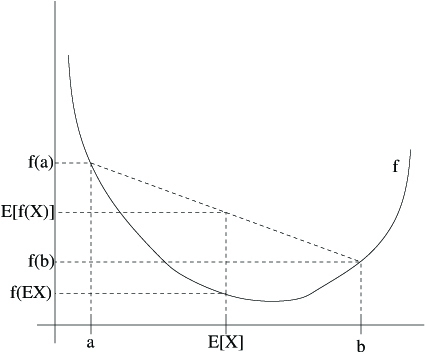
Here, $f$ is a convex function shown by the solid line. Also, $X$ is a random variable that has a $0.5$ chance of taking the value $a$, and a $0.5$ chance of taking the value $b$ (indicated on the $x$-axis). Thus, the value $E(X)$ is given by the midpoint between $a$ and $b$. The value $E[f(X)]$ is now the midpoint on the $y$-axis between $f(a)$ and $f(b)$. We see that because $f$ is convex, it must be the case that $E[f(X)] ≥ f(EX)$.

Derivation of EM Algorithm

The expectation-maximization (EM) algorithm is a very general iterative algorithm for parameter estimation (model fitting) by maximum likelihood, when some of data (random variables) involved are not observed, i.e. missing or incomplete. These unobservable variables are usually called as latent variables.

Suppose there are latent variables $z_i$’s ($z_i$ can be a scalar or vector). For each $i$, let $q_i(\cdot)$ be the probability distribution function of the random variable $z_i$. Denote \(X:= (x_1, \cdots, x_n)^T, Z := (z_1, \cdots, z_n)^T\), where $X$ is observable data and $Z$ is unobservable (hidden, missing) data.

We wish to fit the parameters $\theta$ of a model $p(x;\theta)$ to the observable data $x$. We estimate the parameters $\theta$ by maximizing the log likelihood.

Note: There are two different approaches to derive the EM algorithm. The following is the approach that was introduced by Andrew Ng in his lecture notes.

If $z_i$ is a continuous random variable. The log likelihood for the observable data $x_i$’s is

\[\begin{align*} \ell(X; \theta) &= \log L(X; \theta) \\ &= \sum_{i=1}^n \log p(x_i;\theta) \\ &= \sum_{i=1}^n \log \sum_{z_i} p(x_i, z_i; \theta) \\ &= \sum_{i=1}^n \log \sum_{z_i} q_i(z_i) \frac{p(x_i, z_i; \theta)}{q_i(z_i)} \\ &= \sum_{i=1}^n \log E_{z_i \sim q_i} \Big[\frac{p(x_i, z_i; \theta)}{q_i(z_i)} \Big] \\ & \geq \sum_{i=1}^n E_{z_i \sim q_i} \bigg[ \log \frac{p(x_i, z_i; \theta)}{q_i(z_i)} \bigg] \\ &= \sum_{i=1}^n \sum_{z_i} q_i(z_i) \log \frac{p(x_i, z_i; \theta)}{q_i(z_i)}. \tag{1} \end{align*}\]

where the “\(z_i \sim q_i\)” subscripts above indicate that the expectations are with respect to $z_i$ drawn from $q_i$.

The last second step of the derivation above used Jensen’s inequality. Since $f(\cdot) = \log(\cdot)$ is a concave function, by Jensen’s inequality, we have

\[f \bigg( E_{z_i \sim q_i} \Big[\frac{p(x_i, z_i; \theta)}{q_i(z_i)} \Big] \bigg) \geq E_{z_i \sim q_i} \bigg[ f \Big( \frac{p(x_i, z_i; \theta)}{q_i(z_i)} \Big) \bigg]. \tag{2}\]

Define

\[J(\mathbf{q},\theta) = J(q_1,\cdots,q_n, \theta) := \sum_{i=1}^n E_{z_i \sim q_i} \bigg[ \log \frac{p(x_i, z_i; \theta)}{q_i(z_i)} \bigg] = \sum_{i=1}^n \sum_{z_i} q_i(z_i) \log \frac{p(x_i, z_i; \theta)}{q_i(z_i)}.\]

Now, for any set of distributions $\mathbf{q}$, the formula (1) gives a lower-bound \(J(\mathbf{q},\theta)\) on the log likelihood $\ell(\theta)$.

To increase the lower bound of $\ell(\theta)$ as much as possible, it seems natural to select $\mathbf{q}$ ($q_i$’s) that makes the lower-bound tight at that value of $\theta$. I.e., we’ll make the inequality hold with equality at our particular value of $\theta$. To do that, we need to make the Jensen’s inequality in equitation (2) to hold with equality, which means \(\frac{p(x_i, z_i; \theta)}{q_i(z_i)}\) need to be a constant-valued random variable.

Thus, to get the tight lower bound on $\ell(\theta)$, we require that \(\frac{p(x_i, z_i; \theta)}{q_i(z_i)} = c\) for some constant $c$ that does not depend on $z_i$. Since \(1 = \sum_{z_i} q_i(z_i) = \sum_{z_i} \frac{1}{c} p(x_i, z_i; \theta) = \frac{1}{c} \sum_{z_i} p(x_i, z_i; \theta)\), we have \(c = \sum_{z_i} p(x_i, z_i; \theta)\). It follows that

\[q_i(z_i) = \frac{ p(x_i, z_i; \theta)} {\sum_{z_i} p(x_i, z_i; \theta) } = \frac{ p(x_i, z_i; \theta)} {p(x_i; \theta)} = p(z_i | x_i; \theta).\]

Therefore, we simply set the $q_i$ to be the posterior distribution of the $z_i$ given $x_i$ and the setting of the parameters $\theta$, which is denoted as $\theta^{(t)}$ at $t$-th iteration.

At $t$-th step, $\mathbf{q}^{(t)}$ and \(\theta^{(t)}\) are known. By the equation (1), we have

\[\ell(\theta^{(t+1)}) \geq J(\mathbf{q}^{(t)}, \theta^{(t)}). \tag{3}\]

At $t$-th iteration of the EM algorithm, for the choice of the $q_i^{(t+1)}$’s, the equation (3) gives a lower bound on the loglikelihood that we’re trying to maximize. We select \(q_i^{(t+1)}(z_i) = p(z_i \mid x_i; \theta^{(t)})\) to make the lower bound tight, then we have $\ell(\theta^{(t+1)}) = J(\mathbf{q}^{(t+1)}, \theta^{(t)})$. This is the E-step.

In the M-step of the algorithm, we then maximize the tight lower bound

\[J(\mathbf{q}^{(t+1)}, \theta^{(t)}) = \sum_{i=1}^n \sum_{z_i} q_i^{(t+1)}(z_i) \log \frac{p(x_i, z_i; \theta)}{q_i^{(t+1)}(z_i)} = \sum_{i=1}^n \sum_{z_i} p(z_i \mid x_i; \theta^{(t)}) \log \frac{p(x_i, z_i; \theta)}{p(z_i \mid x_i; \theta^{(t)})}\]

with respect to the parameters $\theta$ to obtain a new setting of the parameters, which is $\theta^{(t+1)}$.

Algorithm. EM algorithm:

[1] Initialize the value of $\theta$ as $\theta^{(0)}$.

[2] Repeat these two steps until convergence:

(a) E-step. For each \(i\), set \(q_i^{(t+1)}(z_i) := p(z_i \mid x_i; \theta^{(t)})\);

(b) M-step. Update \(\theta^{(t+1)} := \underset{\theta}{\text{argmax }} J(\mathbf{q}^{(t+1)}, \theta^{(t)}) = \underset{\theta}{\text{argmax }} \sum_{i=1}^n \sum_{z_i} p(z_i \mid x_i; \theta^{(t)}) \log \frac{p(x_i, z_i; \theta)}{p(z_i \mid x_i; \theta^{(t)})}\).

Remark. The EM algorithm can also be viewed a coordinate ascent on $J(\mathbf{q}, \theta)$, in which the E-step maximizes it with respect to $\mathbf{q}$, and the M-step maximizes it with respect to $\theta$.

Summary:

\[\newcommand{\vc}[3]{\overset{#2}{\underset{#3}{#1}}} \ell(\theta^{(t+1)}) \geq J(\mathbf{q}^{(t)}, \theta^{(t)}) \vc{\implies}{\text{E-step}}{\text{Update } \mathbf{q}} \ell(\theta^{(t+1)}) = J(\mathbf{q}^{(t+1)}, \theta^{(t)}) \vc{\implies}{\text{M-step}}{\text{Update } \theta} \ell(\theta^{(t+2)}) \geq J(\mathbf{q}^{(t+1)}, \theta^{(t+1)}) \vc{\implies}{\text{E-step}}{\text{Update } \mathbf{q}} \cdots\]

Denote \(Q(\theta;\theta^{(t)}) := \sum_{i=1}^n \sum_{z_i} p(z_i \mid x_i; \theta^{(t)}) \log p(x_i, z_i; \theta)\).

We have \(\underset{\theta}{\text{argmax }} \sum_{i=1}^n \sum_{z_i} p(z_i \mid x_i; \theta^{(t)}) \log \frac{p(x_i, z_i; \theta)}{p(z_i \mid x_i; \theta^{(t)})} = \underset{\theta}{\text{argmax }} Q(\theta;\theta^{(t)})\). To derive the other form of the algorithm, note that

\[\begin{align*} Q(\theta;\theta^{(t)}) &= \sum_{i=1}^n \sum_{z_i} p(z_i \mid x_i; \theta^{(t)}) \log p(x_i, z_i; \theta) \\ &= \sum_{i=1}^n E_{z_i \mid x_i;\theta^{(t)}} \Big[\log p(x_i,z_i;\theta) \mid x_i \Big] \\ &= E_{Z \mid X;\theta^{(t)}} \Big[ \sum_{i=1}^{n} \log p(x_i,z_i;\theta) \mid X \Big] \\ &= E_{Z \mid X; \theta^{(t)}} \Big[ \ell(X, Z ; \theta) \mid X \Big]. \end{align*}\]

Remark. The algorithm can also be written as

(a) E-step. Set \(Q(\theta;\theta^{(t)}) := \sum_{i=1}^n \sum_{z_i} p(z_i \mid x_i; \theta^{(t)}) \log p(x_i, z_i; \theta) = E_{Z \mid X;\theta^{(t)}} \Big[ \ell(X,Z ; \theta) \mid X \Big]\).

(b) M-step. Update \(\theta^{(t+1)} := \underset{\theta}{\text{argmax }} Q(\theta;\theta^{(t)})\).

Gaussian Mixture Model

The mixture models can be used for clustering problems. We assume observations in the same cluster follow the same distribution, while observations in different clusters follow different distributions. For Gaussian mixture model, we assume the observations follow the Gaussian distributions.

These assumptions can be written as \(x_i \mid z_{ik}=1 \sim N(\mu_k, \Sigma_k)\) for every \(i\), where \(z_{ik} = 1\) if \(x_i\) is from $k$-th cluster and \(z_{ik} = 0\) otherwise. Here, \(z_i\text{'s} \overset{\text{i.i.d.}}{\sim} \text{Multinoulli}(\pi)\), where \(\mathbf{\pi} = (\pi_1, \cdots, \pi_K)^T \in \mathbb{R}^K\) and \(\sum_{k=1}^K \pi_k = 1\). Note that $z_i$’s are latent random variables, which are hidden and unobservable.

We want to estimate the parameters \(\mathbf{\pi}\), \(\mathbf{\mu}\) and \(\mathbf{\Sigma}\) (i.e. \(\pi_1,\cdots,\pi_K,\mu_1,\cdots,\mu_K,\Sigma_1,\cdots,\Sigma_K\)). To estimate them, we first written down the loglikelihood of the observable data $x_i$’s:

\[\begin{align*} \ell(\mathbf{\pi}, \mathbf{\mu}, \mathbf{\Sigma}) &= \log L(\mathbf{\pi}, \mathbf{\mu}, \mathbf{\Sigma}) \\ &= \sum_{i=1}^n \log p(x_i;\mathbf{\pi}, \mathbf{\mu}, \mathbf{\Sigma}) \\ &= \sum_{i=1}^n \log \sum_{z_i} p(x_i, z_i; \theta). \end{align*}\]

Since there are latent variables $z_i$’s, let’s apply EM algorithm.

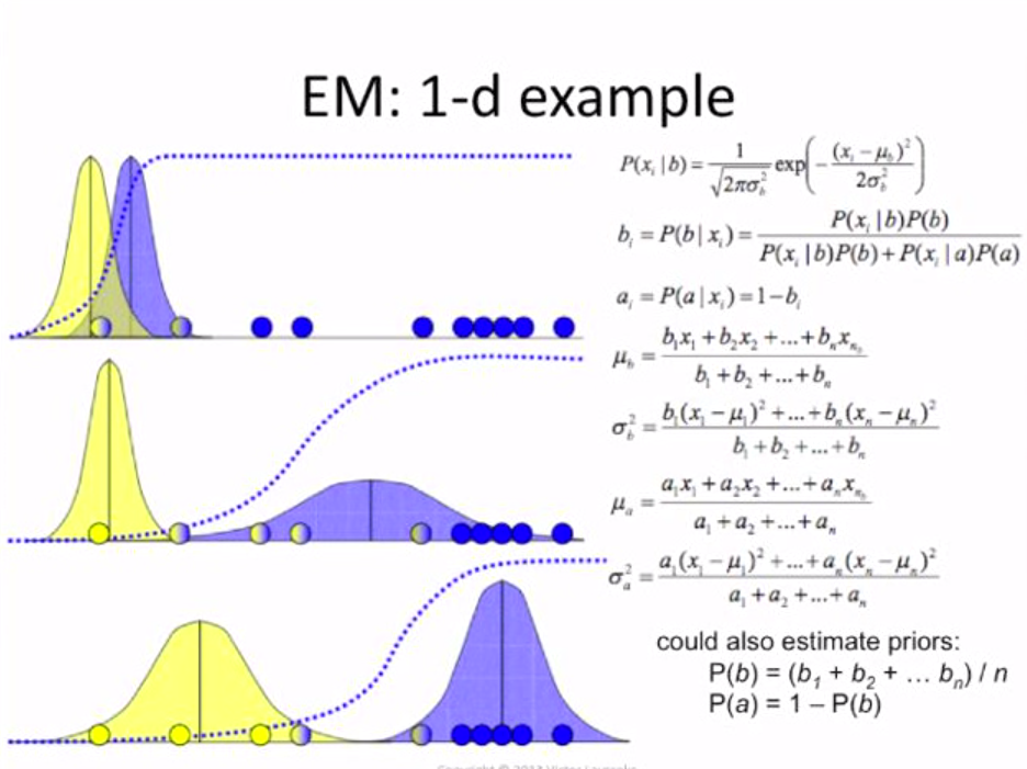
E-step: For each $i,k$, set $w_{ik} := q_i(z_{ik}=1) = P(z_{ik}=1 \mid x_i; \mathbf{\pi}, \mathbf{\mu}, \mathbf{\Sigma})$;

M-step: For each $k$, update the parameters

\[\pi_k := \frac{1}{n} \sum_{i=1}^{n} w_{ik}, \\ \mu_k := \frac{\sum_{i=1}^{n} w_{ik} x_i}{\sum_{i=1}^{n} w_{ik}}, \\ \Sigma_k := \frac{\sum_{i=1}^{n} w_{ik} (x_i-\mu_k)(x_i-\mu_k)^T}{\sum_{i=1}^{n} w_{ik}}.\]

In the E-step, \(q_i(z_{ik}=1)\) denotes the probability of $z_{ik}=1$ under the distribution $q_i$, which is \(\text{Multinoulli}(\pi)\). We calculate \(P(z_{ik}=1 \mid x_i; \pi_k, \mu_k, \Sigma_k)\) by using Bayes rule:

\[\begin{align*} P(z_{ik}=1 \mid x_i; \mathbf{\pi}, \mathbf{\mu}, \mathbf{\Sigma}) &= \frac{p(z_{ik}=1,x_i; \mathbf{\pi}, \mathbf{\mu}, \mathbf{\Sigma})}{p(x_i; \mathbf{\pi}, \mathbf{\mu}, \mathbf{\Sigma})} \\ &= \frac{p(x_i \mid z_{ik}=1; \mathbf{\mu}, \mathbf{\Sigma}) P(z_{ik}=1; \mathbf{\pi})} { \sum_{l=1}^{K} p(x_i \mid z_{il}=1 ; \mathbf{\mu}, \mathbf{\Sigma}) P(z_{il}=1; \mathbf{\pi})}. \end{align*}\]

Here, \(p(x_i \mid z_{ik}=1; \mathbf{\mu}, \mathbf{\Sigma})\) is given by evaluating the density of a Gaussian with mean $\mu_k$ and covariance \(Σ_k\) at \(x_i\); \(P(z_{ik}=1; \mathbf{\pi})\) is given by \(\pi_k\). The values \(w_{ik}\) calculated in the E-step represent our “soft” guesses for the probability of \(z_{ik}=1\), which is also the probability of observation \(x_i\) is from $k$-th cluster.

The term “soft” refers to our guesses being probabilities and taking values in \([0,1]\); in contrast, a “hard” guess is one that represents a single best guess (such as taking values in \(\{0,1\}\) or \(\{1,\cdots,k\}\)). EM algorithm makes the “soft” guesses $w_i$ for each observation $i$, while K-means makes the hard guesses \(c_i\).

Similar to K-means, it is also susceptible to local optima, so reinitializing at several different initial parameters may be a good idea.

References:

Andrew Ng. “CS229 Lecture notes: 7a, 7b, 8.”, http://cs229.stanford.edu/notes.

Victor Lavrenko. “Expectation Maximization: how it works”, https://youtu.be/iQoXFmbXRJA.