Image Edge Basis

Goal and Motivation for Edge Detection

The goal of edge detection is to identify sudden changes (discontinuities) in an image. Intuitively, most semantic and shape information from the image can be encoded in the edges, and the edges are more compact than original pixels. The edges help us extract information, recognize objects, and recover the geometry and viewpoint of an image.

Origin of Edges

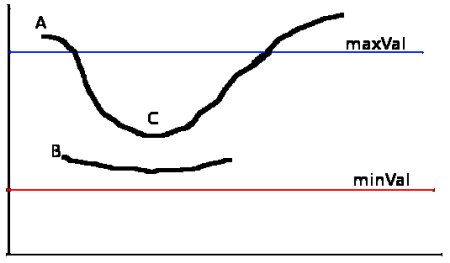
There are four possible sources of edges in an image: surface normal discontinuity (surface changes direction sharply), depth discontinuity (one surface behind another), surface color discontinuity (single surface changes color), illumination discontinuity (shadows/lighting). These discontinuities are demonstrated in the plot below.

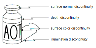
Image Gradients

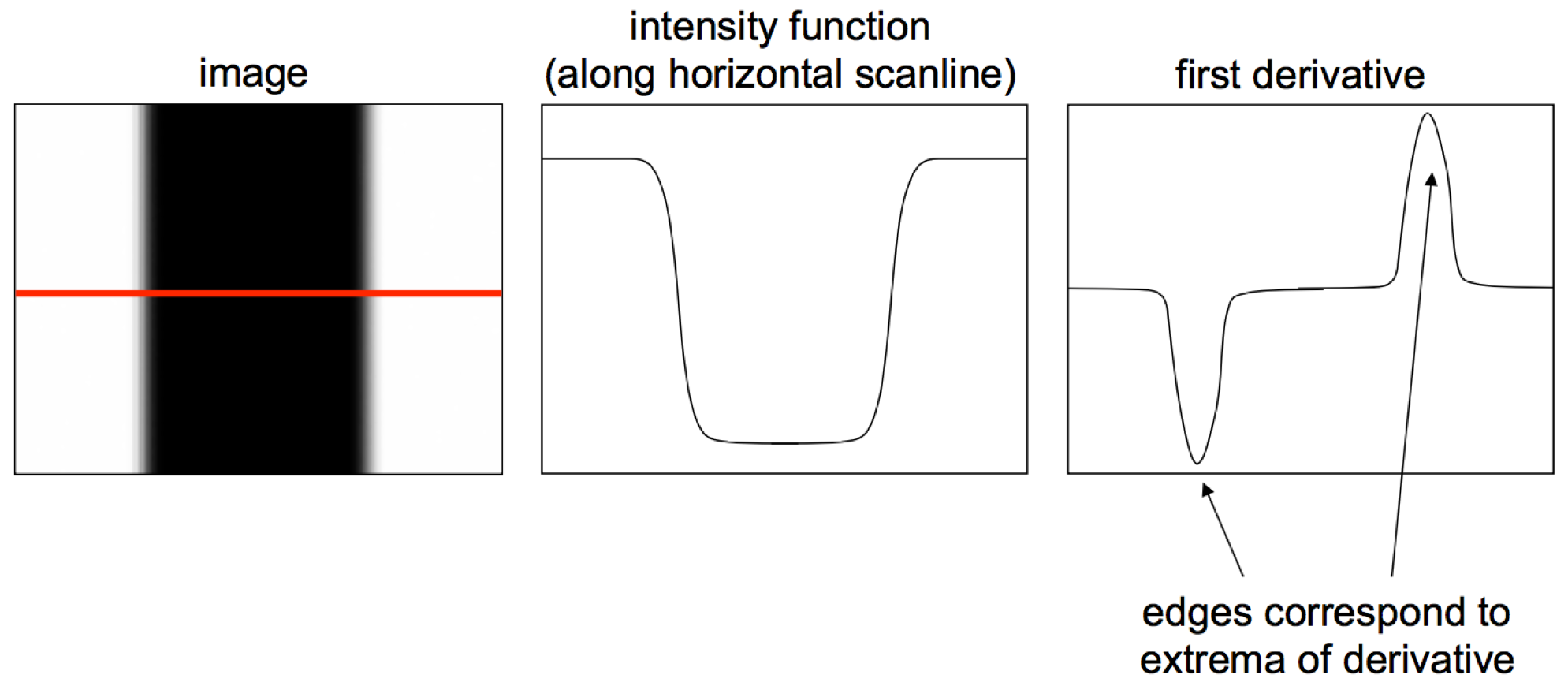
An edge in an image is an image contour across which the image’s brightness or hue changes abruptly. We define an edge as a rapid place of change in the image intensity function, i.e. edges occur in an image when the magnitude of the gradient (first derivative) is high, as shown below.

Discrete Derivatives

There are three main types of derivatives that can be applied on pixels. Their formulas and corresponding filters (convoluting the filter with the image gives the derivatives) are:

\[\begin{aligned} &\text {Backward: } & f^{\prime}(x) &= f(x)-f(x-1) &\rightarrow & \ [0,1,-1], \\ &\text {Forward: } & f^{\prime}(x) &= f(x)-f(x+1) &\rightarrow & \ [-1,1,0], \\ &\text {Central: } & f^{\prime}(x) &= f(x+1)-f(x-1) &\rightarrow & \ \frac{1}{2}[1,0,-1]. \end{aligned}\]

The 2D gradient $ (\nabla f) $ can be calculated as follows:

\[\begin{aligned} \nabla f(x, y) &=\left[\begin{array}{l} \frac{\partial f(x, y)}{\partial x} \\ \frac{\partial f(x, y)}{\partial y} \end{array}\right] = \left[\begin{array}{l} f_{x} \\ f_{y} \end{array}\right]. \end{aligned}\]

We can also calculate the magnitude and the angle of the gradient:

\[\begin{aligned} & \mid\nabla f(x, y)\mid = \sqrt{f_{x}^{2}+f_{y}^{2}}, \\ & \theta =\tan ^{-1}\left(f_{y} / f_{x}\right). \end{aligned}\]

The gradient vectors point toward the direction of the most rapid increase in intensity.

Noise Reduction

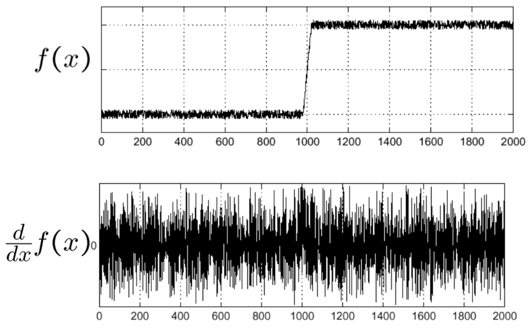
If there is excessive noise in an image, the partial derivatives will not be effective for identifying the edges, as shown below. In order to properly extract edge locations, the noise removal should be preceded before the computing image gradients.

Derivative of Gaussian Filter

We can apply the Gaussian smoothing before computing image gradients.

Let $ f $ and $ h $ be an image and a filter, respectively. Note that one characteristic of convolution is that the derivative of convolved image $ (h * f) $ is equivalent to convolving image $ f $ with the differentiated filter $ \nabla h $.

\[\frac{\partial}{\partial x}(h * f)=\left(\frac{\partial}{\partial x} h\right) * f\]

Using this, we can simplify one operation in previous figure. This time, we first compute the differentiated filter $ \nabla h $ and convolve it with the image $f$, and this yields the same result as that is previous figure.

Smoothing removes noise but blurs edges. Smoothing with different kernel sizes can detect edges at different scales.

Sobel Filter

This algorithm utilizes two $3 \times 3 $ kernels which, once convolved with the image, approximate the $ x $ and $ y $ derivatives of the original image.

\[h_{x}=\left[\begin{array}{ccc} 1 & 0 & -1 \\ 2 & 0 & -2 \\ 1 & 0 & -1 \end{array}\right], \quad h_{y}=\left[\begin{array}{ccc} 1 & 2 & 1 \\ 0 & 0 & 0 \\ -1 & -2 & -1 \end{array}\right].\]

These matrices represent the result of smoothing and differentiation

\[h_{x}=\left[\begin{array}{lll} 1 & 0 & -1 \\ 2 & 0 & -2 \\ 1 & 0 & -1 \end{array}\right]=\left[\begin{array}{l} 1 \\ 2 \\ 1 \end{array}\right]\left[\begin{array}{lll} 1 & 0 & -1 \end{array}\right].\]

The Sobel filter can also be thought of as $3 \times 3$ approximations to first derivative of Gaussian kernels. This approximation enables the Sobel operator to be computed quite quickly, while Gaussian derivatives might be more accurate.

The Sobel Filter has many problems, including poor localization. The Sobel Filter also favors horizontal and vertical edges over oblique edges

Canny Edge Detector

The Canny edge Detector has five algorithmic steps:

1. Suppress noise and compute gradients: Filter image with derivative of Gaussian or Sobel filter;
2. Compute gradient magnitude and direction;
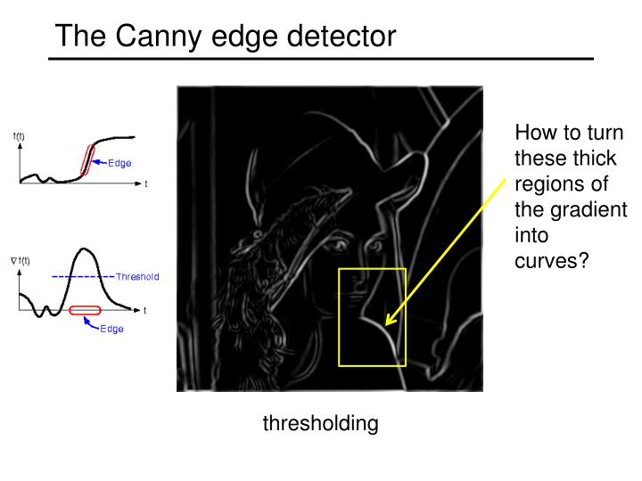
3. Non-maximum suppression: Thin wide “edges” down to single pixel width;
4. Hysteresis thresholding: Use two thresholds to find weak and strong edges;
5. Connectivity analysis to detect edges: Keep strong edges and connect weak edges with them.

Suppress Noise and Compute Gradients

We can both suppress noise and compute the graidents in the x and y directions using methods like derivative of Gaussian filter or Sobel filter.

Compute Gradient Magnitude and Direction

\[\begin{aligned} & \mid\nabla f(x, y)\mid = \sqrt{f_{x}^{2}+f_{y}^{2}}, \\ & \theta =\tan ^{-1}\left(f_{y} / f_{x}\right). \end{aligned}\]

Non-Maximum Suppression

The solution is to check if a pixel is local maximum along gradient direction. Basically, if the pixel is not the largest of the three pixels in the direction and opposite the direction of its gradient, then the gradient of this pixel is set to $0$.

Hysteresis Thresholding

All remaining pixels are subjected to hysteresis thresholding. This part uses two values, for the high and low thresholds. Every pixel with a intensity gradient magnitude above the high threshold is marked as a strong edge. Every pixel below the low threshold is set to non-edge. Every pixel between the two thresholds is marked as a weak edge.

Connectivity Analysis

The final step is connecting the edges. All strong edge pixels are edges. For weak edge pixels, only the weak edge pixels that are linked to strong edge pixels are edges. The part uses BFS (breadth-first search) or DFS (depth-first search) to find all the edges.

References:

CS131 - Computer Vision: Lecture 5

CS131 - Computer Vision: Lecture 6

CS 543/ECE 549 - Computer Vision: Edge detection

OpenCV-Python Tutorials: Canny Edge Detection

Gradient and Laplacian Filter, Difference of Gaussians (DOG)