Tree-based methods partition the feature space into a set of rectangles, and then fit a simple model (like a constant) in each one. They are conceptually simple yet powerful.

1. Regression Trees

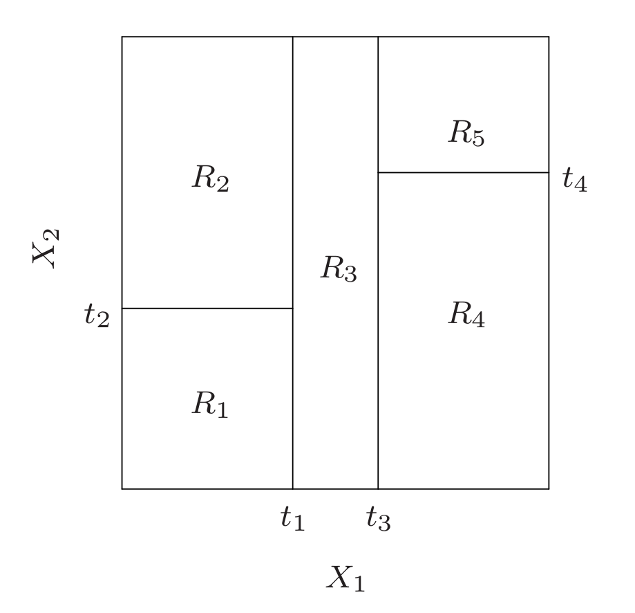
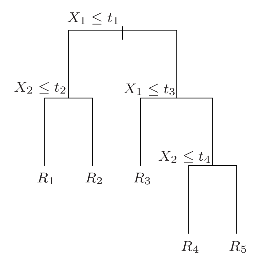
Suppose first that we have a partition into \(M\) regions $R_1, R_2 , …, R_M$ , and we model the response as a constant $c_m$ in each region:

\[f(x) = \sum_{m=1}^{M} c_m \mathbf{1}(x \in R_m ).\]

If we adopt as our criterion minimization of the sum of squares $(y_i −f (x_i )) ^2$, it is easy to see that the best $\hat{c}_m$ is just the average of $y_i$ in region $R_m$: $\hat{c}_m = \text{avg}(y_i \mid x_i ∈ R_m )$.

1.1 How to build a regression tree?

Now finding the best binary partition in terms of minimum sum of squares is generally computationally infeasible. Hence we proceed with a greedy algorithm. Starting with all of the data, consider a splitting variable \(j\) and split point \(s\), and define the regions of left and right node as

\[R_L(j, s) = \{X \mid X_j \leq s\},\ R_R(j, s) = \{X \mid X_j > s\}.\]

The node splitting criteria is that, we seek the splitting variable $j$ and split point $s$ that solve

\[\min_{j,s}\Big[\min_{c_L}\sum_{x_i \in R_L(j,s)} (y_i-c_L)^2 + \min_{c_R}\sum_{x_i \in R_R(j,s)} (y_i-c_R)^2 \Big].\]

For any choice $j$ and $s$, the inner minimization is solved by

\[\hat{c}_L = \text{avg}(y_i \mid x_i \in R_L (j,s)),\ \hat{c}_R = \text{avg}(y_i \mid x_i \in R_R (j, s)).\]

We index nodes by $m$, with node $m$ representing region $R_m$. Letting

\[N_m = \# \{x_i ∈ R_m \}, \\ \hat{c}_m = \frac{1}{N_m} \sum_{x_i\in R_m} y_i, \\ Q_m = \frac{1}{N_m} \sum_{x_i\in R_m} (y_i-\hat{c}_m)^2,\]

where $Q_m$ is the node impurity, and is measured by squared loss.

Denote \(m_L\) and \(m_R\) as the two child nodes created by splitting node \(m\). Then the node splitting criteria can be written as

\[\operatorname*{argmin}_{j,s}\left(N_{m_L}Q_{m_L} + N_{m_R}Q_{m_R} \right).\]

1.2 How to decide the tree size?

We first grow a large tree $T_0$, stopping the splitting process only when some minimum node size (say \(5\)) is reached. Then this large tree is pruned using cost-complexity pruning.

Either the number of leaf nodes or the depth can be used to measure the complexity of a tree. Here we take the previous one for example.

We define a subtree $T ⊂ T_0$ to be any tree that can be obtained by pruning $T_0$, that is, collapsing any number of its internal (non-terminal) nodes. Let $\mid T \mid$ denote the number of terminal nodes in $T$, which refers to the complexity of the tree.

We define the cost complexity criterion for a tree \(T\) as

\[C_\alpha(T) = \sum_{m=1}^{|T|}N_m Q_m + α|T| = \sum_{m=1}^{|T|}\sum_{x_i\in R_m} (y_i-\hat{c}_m)^2 + α|T|,\]

where \(m\) is the index of terminal node, and \(\alpha\) is the regularization parameter (or strength).

The tuning parameter $α ≥ 0$ governs the trade-off between tree size and its goodness of fit to the data. The idea is to find, for each $α$, the subtree $T_α ⊆ T_0$ to minimize $C_α (T )$.

Large values of $α$ result in smaller trees $T_α$, and conversely for smaller values of \(α\). As the notation suggests, with $α$ = 0 the solution is the full tree $T_0$.

For each \(\alpha\) one can show that there is a unique smallest subtree $T_α$ that minimizes $C_α(T)$. For each $\alpha$, to find $T_α$, we use weakest link pruning: we successively collapse the internal node that produces the smallest per-node increase in $\sum_mN_mQ_m$, and continue until we produce the single-node (root) tree. This gives a (finite) sequence of subtrees, and one can show this sequence must contain $T_α$.

To choose $\alpha$, we use cross-validation: we choose the value $\hat{\alpha}$ to minimize the cross-validated loss. Our final tree is $T_\hat{\alpha}$.

2. Classification Trees

The only difference between regression trees and classification trees are the methods of splitting nodes and pruning the tree. In a node $m$, representing a region $R_m$ with $N_m$ observations. The proportion of class $k$ observations in node $m$:

\[\hat{p}_{mk} = \frac{1}{N_m} \sum_{x_i \in R_m} I(y_i=k)\]

We classify the observations in node $m$ to the majority class in node $m$:

\[k(m) = \operatorname*{argmax}_k \hat{p}_{mk}.\]

Different measures $Q_m$ of the impurity of node \(m\) include the following:

\[\text{Misclassification error: } 1-\hat{p}_{mk(m)} = \frac{1}{N_m} \sum_{x_i \in R_m} I(y_i \neq k(m)). \\\text{Gini index: } \sum_{k=1}^{K} \hat{p}_{mk} (1-\hat{p}_{mk}). \\\text{Entropy or deviance: } −\sum_{k=1}^{K} \hat{p}_{mk} \log(\hat{p}_{mk}).\]

For binary classification:

\[\text{Misclassification error: } \frac{1}{2} - \mid \hat{p}_{m1}-\frac{1}{2} \mid. \\\text{Gini index: } 2 \hat{p}_{m1} (1-\hat{p}_{m1}). \\\text{Entropy or deviance: } - \hat{p}_{m1} \log(\hat{p}_{m1}) - (1-\hat{p}_{m1}) \log(1-\hat{p}_{m1}).\]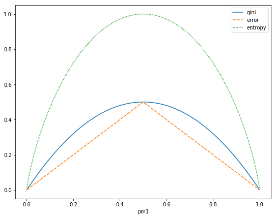

All three are similar, but entropy and the Gini index are differentiable, and hence more amenable to numerical optimization.

Similar to regression tree, the node splitting criteria is that, finding the splitting variable $j$ and split point $s$ by

\[\operatorname*{argmin}_{j,s}\left(N_{m_L}Q_{m_L} + N_{m_R}Q_{m_R} \right).\]

We can also define a criteria called gain to measure the reduction in impurity after splitting, such as information gain that measures the reduction in entropy.

We select the feature and splitting point for a node that maximize the gain. After splitting the node $m$ to two child nodes $m_L$ (left node) and $m_R$ (right node), we can calculate the gain as

\[\text{Gain}_m = Q_m - \frac{N_{m_L}}{N_m} Q_{m_L} - \frac{N_{m_R}}{N_m} Q_{m_R}.\]

Then the node splitting criteria can be written as

\[\operatorname*{argmin}_{j,s} \text{Gain}_m.\]

Gini index and entropy are more sensitive to changes in the node probabilities than the misclassification rate. For example, in a two-class problem with 400 observations in each class (denote this by (400, 400)), suppose one split created nodes (300, 100) and (100, 300), while the other created nodes (200, 400) and (200, 0). Both splits produce a misclassification rate of 0.25, but the second split produces a pure node and is probably preferable. Both the Gini index and entropy are lower for the second split.

For this reason, either the Gini index or entropy should be used when growing the tree. To guide cost-complexity pruning, any of the three measures can be used, but typically it is the misclassification rate.

Growing a tree: Gini index, entropy. Cost-complexity pruning: any of the three.

We usually treat the class proportions in the terminal node as the class probability estimates.

3. Interpretation

Single decision trees can be graphed and are highly interpretable, but the ensemble trees must be interpreted in the different ways as follow. The following methods can be used for both single tree and ensemble trees.

3. 1 Relative Importance of Predictor Variables

For a single decision tree $T_m$, the importance of the variable \(X_j\) (denote as \(\mathcal{I}_j^2(T_m)\)) can be measured by the sum of the improvements in loss after partition regions by variable $X_j$ over all nodes.

For additive tree expansions, it is simply averaged over the trees \(\mathcal{I}_j^2 = \frac{1}{M} \sum_{m=1}^{M} \mathcal{I}_j^2(T_m)\).

3.2 Partial Dependence Plots

Let $\mathcal{S} ⊂ {1,2,…,p}$. Let $\mathcal{C}$ be the complement set of $\mathcal{S}$, with $\mathcal{S} ∪ \mathcal{C} = {1,2,…,p}$. The goal is to produce a visual description of the effect of $X_S$ on $f$ via a plot of $\hat{f}(X_S)$. A general function $f(X)$ will in principle depend on all of the input variables: $f(X) = f(X_\mathcal{S},X_\mathcal{C})$.

The average or partial dependence of $f(X)$ on $X_\mathcal{S}$ can be defined as \(f_\mathcal{S}(X_\mathcal{S}) = E_{X_\mathcal{C}} f (X_\mathcal{S}, X_\mathcal{C})\), and can be estimated by

\[\bar{f}_\mathcal{S}(X_\mathcal{S}) = \frac{1}{N} \sum_{i=1}^{N} f(X_\mathcal{S}, x_\mathcal{iC}),\]

where ${x_{1\mathcal{C}},…,x_{N\mathcal{C}} }$ are the values of $X_\mathcal{C}$ occurring in the training data.

Partial dependence functions \(f_\mathcal{S}(X_\mathcal{S})\) can be used to interpret the results of any “black box” learning method. However, it can be computationally intensive. Fortunately with decision trees, \(\bar{f}_\mathcal{S}(X_\mathcal{S})\) can be rapidly computed from the tree itself without reference to the data (ESL Exercise 10.11).

The partial dependence of $f(X)$ on $X_\mathcal{S}$ is a marginal average of $f$, and can represent the effect of $X_\mathcal{S}$ on $f(X)$ after accounting for the (average) effects of the other variables $X_\mathcal{C}$ on $f(X)$. It is not the effect of \(X_\mathcal{S}\) on $f(X)$ ignoring the effects of $X_\mathcal{C}$. The latter is given by the conditional expectation \(\tilde{f}_\mathcal{S}(X_\mathcal{S}) = E[f(X_\mathcal{S}, X_\mathcal{C}) \mid f(X_\mathcal{S})]\).

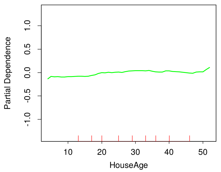
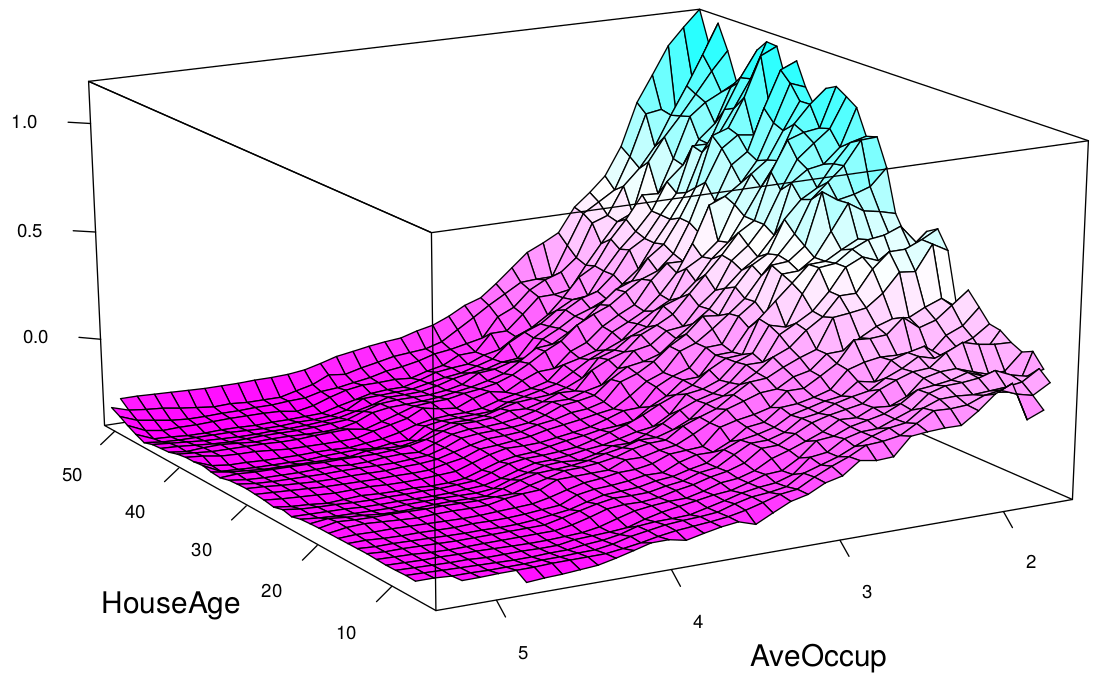
The plots above show the partial dependence of house value on average occupancy and house age. There appears to be a strong interaction effect between these two variables.

4. Some Tips

Time complexity analysis: Suppose we have \(N\) observations with \(p\) features. Splitting a non-leaf node with \(N_m\) observations costs \(N_mp\) time, and the total number of observations in each level of the tree is \(N\), and it follows that the training time costs in each level are all \(Np\). Thus the time complexity of training a tree of depth \(d\) is \(O(Npd)\). If every leaf node contains one observation, then \(d=\log_2N\) in the best case of a balanced tree and \(d=N-1\) in the worst case of a skewed tree. Also obviously, the prediction time complexity for a input is \(O(d)\).

A key advantage of the recursive binary tree is its interpretability. However, one major problem with trees is their high variance, which makes interpretation somewhat precarious. The major reason for this instability is the hierarchical nature of the process: the effect of an error in the top split is propagated down to all of the splits below it. Bagging averages many trees to reduce the variance.

Tree or ensemble tree methods are not suitable for high dimensional sparse data. (Explanation in Chinese)

Some aspects of decision tree learning:

• Time complexity (\(N\): number of observations; \(p\): number of features; \(d\): depth of the tree):
  • Training: \(O(Npd)\);
  • Prediction: \(O(d)\).

• Multi-way splits?

  • fragments the data very quickly;
  • you can always realize a multi-way split by doing a series of binary splits.

• Linear combinations of splits? E.x. $R_1 = {X: 2X_1+X_2 < 0 }, R_2 = {X: 2X_1+X_2 \geq 0 }$ .

  • maybe good for prediction;
  • not good for interpretation;
  • expensive for computation.

• What types of functions does regression tree have trouble approximating?

  • additive function $f(X) = \sum_{j=1}^{p} f_j(X_j)$. e.x. $f(X)=\sum_{j=1}^{p} \beta_j X_j$. (note that $Y=f(X)+\epsilon$)
  • $f(X) = I{X_1 \leq t_1 } + I{X_2 \leq t_2 }$.

• Ways to handle missing data

  • remove observations containing missing values;

  • add category “missing” and check whether “missing” has any predictive value;

  • surrogate splits.

Reference:

Friedman, Jerome, Trevor Hastie, and Robert Tibshirani. The elements of statistical learning. Vol. 1. No. 10. New York: Springer series in statistics, 2001.