
Fourier Series
We know that the sum of sinusoidal functions (cosine and sine) will still be a periodic function. However, the Fourier series do the inverse: it breaks down a periodic function into the sum of sinusoidal functions. The Fourier series is the Fourier transform for periodic functions.
Here is an example from Math is fun shows the plot of \(\sin(x)+\sin(2x)\).

Definition
The Fourier series of a periodic function \(f(t)\) with fundamental period \(T\) is
\[\begin{align} f(t) &= \frac{a_0}{2} + \sum_{n=1}^\infty a_n \cos \frac{2\pi nt}{T} + \sum_{n=1}^\infty b_n\sin \frac{2\pi nt}{T}, \end{align}\]where \(t\in\mathbb{R}\) and it is called the time.
Note that it is an equal sign but not approximately equal sign in the formula above, and that means we can approximate $f(t)$ exactly by the Fourier series whenever $f(t)$ is continuous and smooth.
The Fourier coefficients \(\{a_n\}_{n=0}^\infty\) and \(\{b_n\}_{n=1}^\infty\) are
\[a_n = \frac{2}{T} \int_0^T f(t) \cos \frac{2\pi nt}{T} dt, \ \ \ {n = 0,1,\cdots};\\ b_n = \frac{2}{T} \int_0^T f(t) \sin \frac{2\pi nt}{T} dt, \ \ \ {n = 1,2,\cdots}.\]Note that the constant term \(\frac{a_0}{2} = \frac{1}{T} \int_0^T f(t) dt\) is the average value of \(f(t)\) over a period. The intuitive explanation is, if we want to approximate \(f(t)\) by one term \(\frac{a_0}{2}\), the optimal value of \(\frac{a_0}{2}\) is given by the average value of \(f(t)\) over a period.
Complex Form
The previous definition on Fourier series used only real numbers. In engineering, physics and many applied fields, using complex numbers makes things easier to understand and more mathematically elegant. Now let’s introduce the complex form of the Fourier series.
Euler’s formula tells us the complex exponential can be written as a sum of sinusoidal functions. By Euler’s formula, we have
\[e^{ix}=\cos x + i\sin x \implies \cos x = \frac{e^{ix} + e^{-ix}}{2}, \sin x = \frac{e^{ix} - e^{-ix}}{2i},\]where \(x\) is a arbitrary real number and \(i\) is the imaginary unit.
Now let’s derive the complex form of the Fourier series. In this case, we use the complex exponential function as the basis.
\[\begin{align} f(t) &= \frac{a_0}{2} + \sum_{n=1}^\infty \left(a_n \cos \frac{2\pi nt}{T} + b_n\sin \frac{2\pi nt}{T} \right) \\ &= \frac{a_0}{2} + \sum_{n=1}^\infty \left( a_n \frac{e^{i\frac{2\pi nt}{T}} + e^{-i\frac{2\pi nt}{T}}}{2} + b_n \frac{e^{i\frac{2\pi nt}{T}} - e^{-i\frac{2\pi nt}{T}}}{2i} \right) \\ &= \frac{a_0}{2} + \sum_{n=1}^\infty \frac{a_n - ib_n}{2} e^{i\frac{2\pi nt}{T}} + \sum_{n=1}^\infty \frac{a_n + ib_n}{2} e^{-i\frac{2\pi nt}{T}} \\ &= \sum_{n=-\infty}^\infty c_n e^{i\frac{2\pi nt}{T}}, \end{align}\]Thus the complex form of Fourier series of a periodic function \(f(t)\) with period \(T\) is
\[f(t) = \sum_{n=-\infty}^\infty c_n e^{i\frac{2\pi nt}{T}}.\]where
\[c_n = \begin{cases} \frac{a_{-n} + ib_{-n}}{2}, &\text{ if } n<0; \\ \frac{a_0}{2}, &\text{ if } n=0;\\ \frac{a_n - ib_n}{2}, &\text{ if } n>0. \end{cases}\]The complex Fourier coefficients \(\{c_n\}_{n=-\infty}^{\infty}\) are computed as
\[\begin{align} {c_n} &= \frac{1}{T} \int_{0}^T {f\left( t \right){e^{-i\frac{2\pi nt}{T}}}dt}, \\ &= \frac{1}{T} \int_{-\frac{T}{2}}^{\frac{T}{2}} {f\left( t \right){e^{-i\frac{2\pi nt}{T}}}dt}, \ \ \ {n = 0, \pm 1, \pm 2, \cdots }. \end{align}\]Fourier Transform
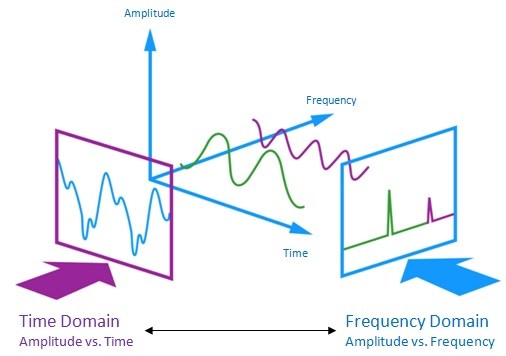
The Fourier transform is a mathematical technique that transforms a function of time, $f(t)$, to a function of frequency, \(\hat{f}(s)\). The Fourier series showed us how to rewrite any periodic function into a sum of sinusoids, while the Fourier transform of an arbitrary function can be derived as a special case of the Fourier series when the period \(T\to\infty\), since that a non-periodic function can be viewed as a limiting case of a periodic function with an infinitely long period.
Derivation
As the period \(T\to\infty\), the quantity \(\frac{2\pi}{T}\) becomes extremely small and the quantity \(\frac{2\pi n}{T}\) becomes a continuous quantity that can take on any value since \(n\) has a range of \((-\infty,+\infty)\). So we define a new variable called the frequency as
\[s := \frac{n}{T}.\]Let
\[\hat{f}(s) := Tc_n = \int_{-\frac{T}{2}}^{\frac{T}{2}} {f\left( t \right){e^{-i\frac{2\pi nt}{T}}}dt} = \int_{-\frac{T}{2}}^{\frac{T}{2}} {f\left( t \right){e^{-2\pi ist}}dt}.\]As \(T\to\infty\), we have the (forward) Fourier transform:
\[\hat{f}(s) = \int_{-\infty}^{\infty} f(t)e^{-2\pi ist}dt.\]Likewise, we can derive the inverse Fourier transform that recover \(f(t)\) from \(\hat{f}(s)\). Start from the complex form of Fourier series, we have
\[f(t) = \sum_{n=-\infty}^\infty c_n e^{i\frac{2\pi nt}{T}} = \sum_{n=-\infty}^\infty Tc_n e^{i\frac{2\pi nt}{T}} \frac{1}{T} = \sum_{n=-\infty}^\infty \hat{f}(s) e^{2\pi ist} \frac{1}{T}.\]The points \(s=\frac{n}{T}\) are spaced \(\frac{1}{T}\) apart, so we can think of \(\frac{1}{T}\) as, say \(\Delta s\), and the sum above as a Riemann sum approximating an integral
\[f(t) = \sum_{n=-\infty}^\infty \hat{f}(s) e^{2\pi ist} \frac{1}{T} = \sum_{n=-\infty}^\infty \hat{f}(s) e^{2\pi ist} \Delta s \approx \int_{-\infty}^{\infty} \hat{f}(s)e^{2\pi ist}ds.\]Thus as \(T\to\infty\), we have the inverse Fourier transform:
\[f(t) = \int_{-\infty}^{\infty} \hat{f}(s)e^{2\pi ist}ds.\]Definition
The Fourier transform of a function $f(t)$ is defined as
\[\hat{f}(s) = \int_{-\infty}^{\infty} f(t)e^{-2\pi ist}dt,\]where \(s\in\mathbb{R}\) and it is called the frequency.
The inverse Fourier transform is then defined as
\[f(t) = \int_{-\infty}^{\infty} \hat{f}(s)e^{2\pi ist}ds.\]The original signal \(f(t)\) is defined on the time domain (or the spatial domain) and the \(\hat{f}(s)\) is defined on the frequency domain. The Fourier transform analyzes a signal into its frequency components. The set of all frequencies is the spectrum of $f(t)$. The value of \(f(t)\) or \(\hat{f}(s)\) is called the amplitude.
Note that for a (non-periodic) signal defined on the whole real line we generally do not have a discrete set of frequencies, as in the periodic case, but rather a continuum of frequencies.
References:
Osgood, Brad. (2007). Lecture Notes for EE261: The Fourier Transform and its Applications. Retrieved July 15, 2020, from https://see.stanford.edu/materials/lsoftaee261/book-fall-07.pdf.
Bevel, Pete. (2010). The Fourier Transform. Retrieved July 17, 2020, from http://www.thefouriertransform.com.
Svirin, Alex. (2020). Complex Form of Fourier Series. Retrieved July 17, 2020, from https://www.math24.net/complex-form-fourier-series.
Cheever, Erik. (2005). Introduction to the Fourier Transform. Retrieved July 18, 2020, from https://lpsa.swarthmore.edu/Fourier/Xforms/FXformIntro.html.