
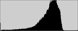
Image Grayscale Histograms
Histograms measure the frequency of brightness within the image: how many times does a particular pixel value appear in an image. A histogram shows the contrast, brightness, intensity distribution etc. of that image.

The pixel intensity is a single value for a grayscale image, or three values for a color image. The histogram above is drawn for grayscale image, not color image.
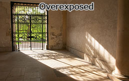
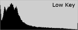
High & Low Key; Over & Under Exposure
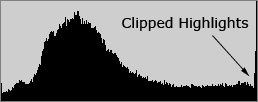
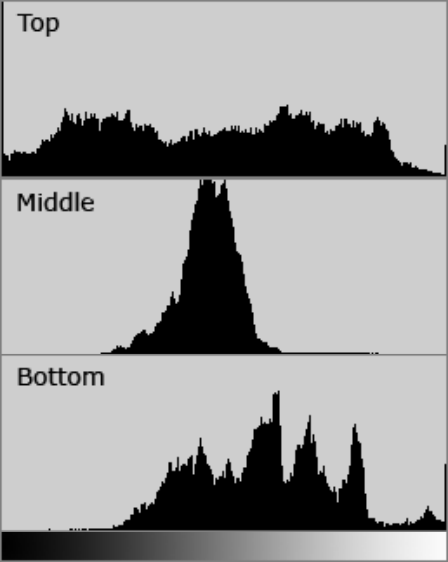
The region where most of the brightness values are present is called the “tonal range”.
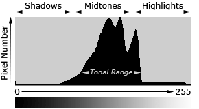
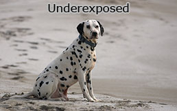
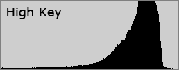
Images where most of the tones occur in the shadows are called “low key,” whereas with “high key” images most of the tones are in the highlights. Most cameras will produce midtone-centric histograms when in an automatic exposure mode.
Contrast
Contrast is a measure of the difference in brightness between light and dark areas in a scene.
Root mean square (RMS) contrast is defined as the standard deviation of the pixel intensities:
\[\sqrt{\frac{1}{W H} \sum_{i=0}^{W-1} \sum_{j=0}^{H-1}\left(I_{i j}-\bar{I}\right)^{2}}\]where intensities \(I_{i j}\) are the \(i\)-th \(j\)-th element of the two-dimensional image of size \(W\) by \(H\). \(\bar{I}\) is the average intensity of all pixel values in the image. The image \(I\) is assumed to have its pixel intensities normalized in the range \([0,1]\).
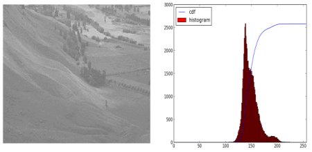
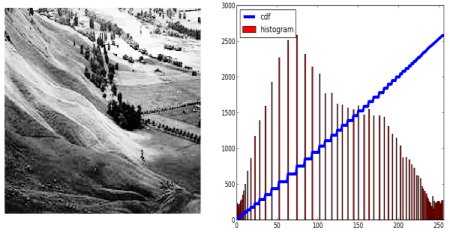
Broad histograms reflect a scene with significant contrast, whereas narrow histograms reflect less contrast. Contrast can have a significant visual impact on an image by emphasizing texture.


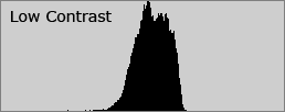
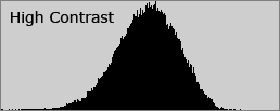
Contrast can also vary for different regions within the same image due to both subject matter and lighting.
Histogram Equalization
Histogram equalization usually increases the contrast of our images, especially when the usable data of the image is represented by close contrast values. Through this adjustment, the intensities can be better distributed on the histogram. Histogram equalization accomplishes this by effectively spreading out the most frequent intensity values.

Let \(f\) be a given image represented as a matrix of integer pixel intensities ranging from \(0\) to \(L-1\). \(L\) is the number of possible intensity values, often \(256\). Let \(p_f(k)\) denote the probability density function (PDF) of the normalized histogram of \(f\) with a bin for each possible intensity \(k\). So
\[p_f(k) = \frac{\text{Number of pixels with intensity } k}{\text{Total number of pixels}}, \quad k=0,1, \cdots, L-1.\]The corresponding cumulative distribution function (CDF) is
\[F_f(l) = \sum_{k=0}^{l} p_f(k).\]The histogram equalized image $ g $ will be defined by
\[g_{i, j} = T_f(f_{i,j}) = \text{floor}\left((L-1) F_f(f_{i,j}) \right) = \text{floor}\left((L-1) \sum_{k=0}^{f_{i, j}} p_f(k)\right)\]where \(T_f(\cdot)\) is the transformation function of the histogram equalization of \(f\), and \(\text{floor}()\) rounds down to the nearest integer. Note that the transformation function \(T_f(\cdot)\) is proportional to the CDF \(F_f(\cdot)\) of \(f\).
The derivation of the transformation function is provided here.
The method is useful in images with backgrounds and foregrounds that are both bright or both dark. In particular, the method can lead to better views of bone structure in X-ray images, and to better detail in photographs that are over or under-exposed. Histogram equalization often produces unrealistic effects in photographs; however it is very useful for scientific images like thermal, satellite or X-ray images.
A key advantage of the method is that it is a fairly straightforward technique and an invertible operator. So in theory, if the histogram equalization function is known, then the original histogram can be recovered. The calculation is not computationally intensive. A disadvantage of the method is that it is indiscriminate. It may increase the contrast of background noise, while decreasing the usable signal.
AHE and CLAHE
Ordinary histogram equalization uses the same transformation derived from the image histogram to transform all pixels. This works well when the distribution of pixel values is similar throughout the image. However, when the image contains regions that are significantly lighter or darker than most of the image, the contrast in those regions will not be sufficiently enhanced, or even weakened.
As shown below, it is true that the background contrast has improved after histogram equalization. But the contrast on the face of statue is weakened and we lost most of the information there due to over-brightness. It is because its histogram is not confined to a particular region.

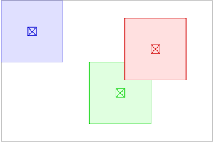
Adaptive histogram equalization (AHE) improves on this by transforming each pixel with a transformation function derived from a neighborhood region, as in the figure below. The derivation of the transformation functions from the histograms is exactly the same as for ordinary histogram equalization.
Ordinary AHE tends to overamplify the contrast in near-constant regions of the image, since the histogram in such regions is highly concentrated. As a result, AHE may cause noise to be amplified in near-constant regions. Contrast Limited AHE (CLAHE) is a variant of adaptive histogram equalization in which the contrast amplification is limited, so as to reduce this problem of noise amplification.
In CLAHE, the contrast amplification in the vicinity of a given pixel value is given by the slope of the transformation function. In another word, the larger of the slope, the larger of the contrast amplification. The slope of the transformation function is proportional to the slope of the neighborhood CDF and therefore to the value of the histogram at that pixel value. CLAHE limits the amplification by clipping the histogram at a predefined limit before computing the CDF. This limits the slope of the CDF and therefore of the transformation function. The value at which the histogram is clipped, the so-called clip limit, depends on the normalization of the histogram and thereby on the size of the neighborhood region.
It is advantageous not to discard the part of the histogram that exceeds the clip limit but to redistribute it equally among all histogram bins, as shown below.
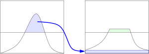
The redistribution will push some bins over the clip limit again (region shaded green in the figure). If this is undesirable, the redistribution procedure can be repeated recursively until the excess is negligible.
The picture below is the result after CLAHE.

References:
Camera Histograms: Tones & Contrast
Wikipedia: Histogram equalization
UCI Math 77C - Image Processing: Histogram Equalization