Imbalanced data typically refers to a problem with classification problems where the classes are not represented equally. This problem can have a significant impact on the effectiveness of the model.

The Effect of Class Imbalance

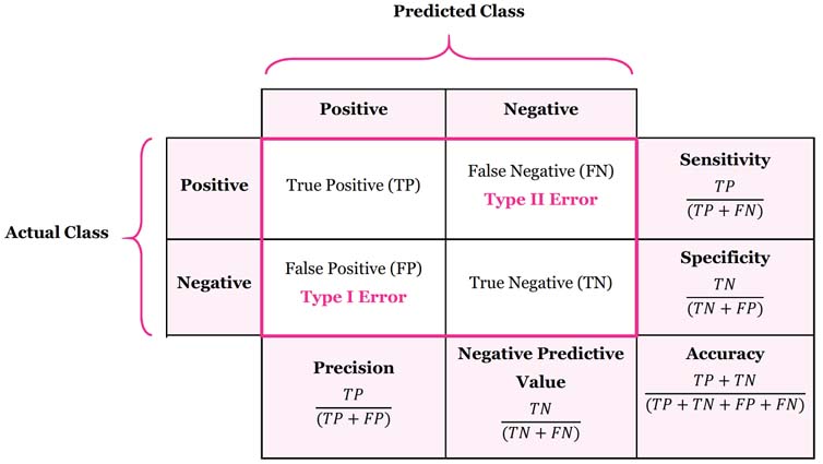
Let’s first review the confusion matrix, as shown below.

Say if we have a imbalanced data set, in which \(99\%\) are of negative class and \(1\%\) are of positive class, then a classification model that always predict “negative” can achieve \(0.99\) accuracy on average. The specificity (true negative rate) of this model is \(\text{TNR} = \frac{TN}{TN+FP} = \frac{99\%}{99\% + 0\%}=1\). However, the sensitivity (true positive rate, or recall) is \(\text{TPR} = \frac{TP}{TP+FN} = \frac{0\%}{0\%+1\%}=0\), which is the fraction of the total amount of positive instances that were actually retrieved.

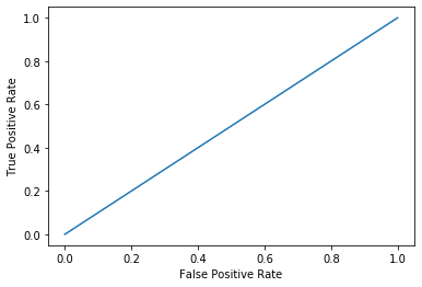
In this case, the ROC curve is a straight line and the AUC is $0.5$, as shown below.

from sklearn.metrics import roc_curve
import matplotlib.pyplot as plt

test = [1] * 100
test[0] = 0
predict = [1] * 100
fpr, tpr, _ = roc_curve(test, predict)
plt.plot(fpr, tpr)
plt.xlabel('False Positive Rate')
plt.ylabel('True Positive Rate')
plt.show()

In the following sections, we discuss the approaches to deal with the class imbalance problems.

Model Selection

Some models like Logistic Regression with loss functions of the form \(\frac{1}{n}\sum_{i=1}^{n}\text{Loss}(\hat{y}_i, y_i)\) are very sensitive to imbalanced dataset. However, models like Decision Tree, Ensemble Trees, and SVM are less sensitive.

As for the tree based methods, the objective of splitting a node is to maximize the information gain and make the sub-nodes as pure as possible, so tree based methods also pay attention to minority class because the minority class can also make the node impure.

As for the SVM, the loss is composed by margin and support vectors, not by all data, thus SVM works well if the support vectors are balanced, and the balanced original dataset is not that necessary.

Changing Performance Metric

Note that the metrics are not the loss functions.

Accuracy is not the metric to use when working with an imbalanced dataset, as we have seen that it is misleading. Instead, we can use F1 score, Cohen’s kappa coefficient, or AUC.

F1 Score

The F1 score is the harmonic mean of the precision and recall (sensitivity), where an F1 score reaches its best value at $1$ (perfect precision and recall). It is defined as

Cohen’s kappa Coefficient

Cohen’s kappa coefficient measures the agreement between two raters. In classification problem, these two raters are true labels and predictions, and the Cohen’s kappa coefficient represents the classification accuracy normalized by the imbalance of the classes in the data. It basically tells you how much better your classifier is performing over the performance of a classifier that simply guesses at random according to the frequency of each class.

The probability of observed agreement is

The probability of expected (random) agreement is

The formula for Cohen’s kappa coefficient is the probability of agreement take away the probability of expected (random) agreement divided by $1$ minus the probability of random agreement:

Cohen’s kappa is always less than or equal to $1$. Values of $0$ or less, indicate that the classifier is useless. There is no standardized way to interpret its values. Landis and Koch (1977) provide a way to characterize values. According to their scheme a value $< 0$ is indicating no agreement, $0\sim0.20$ as slight, \(0.21\sim0.40\) as fair, \(0.41\sim0.60\) as moderate, \(0.61\sim0.80\) as substantial, and \(0.81\sim1\) as almost perfect agreement.

Changing Cutoffs

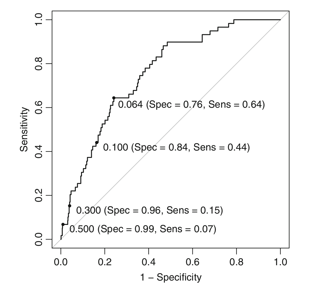
To increase the prediction accuracy of the minority class samples, we can determine alternative cutoffs (or thresholds) for the predicted probabilities. The most straightforward approach is to use the ROC curve since it calculates the sensitivity and specificity across a continuum of cutoffs. Using this curve, an appropriate balance between sensitivity and specificity can be determined.

The plot below is an ROC curve labeled with different probability cutoffs (or thresholds), and the numbers in the parentheses are the specificity and sensitivity.

Several techniques exist for determining a new cutoff. First, if there is a particular target that must be met for the sensitivity or specificity, this point can be found on the ROC curve and the corresponding cutoff can be determined. Another approach for determining a cutoff is to find the point on the ROC curve that is closest (i.e. the shortest distance) to the upper left corner of the plot. Another approach is to find the cutoff associated with the largest value of the Youden’s $J$ index. The index is defined as

In the ROC curve above, we can see that the cutoff $0.064$ is the best with considering either the distance or Youden’s $J$ index.

Note that changing cutoff does not influence the model parameters, and thus it does not increase the overall predictive effectiveness of the model. The main impact that an alternative cutoff has is to make trade-offs between particular types of errors.

References:

Kuhn, M., & Johnson, K. (2013). Remedies for severe class imbalance. In Applied predictive modeling (pp. 419-443). Springer, New York, NY.

Kampakis, S. S. (2016, May 8). Performance Measures: Cohen’s Kappa statistic. The data scientist. Retrieved July 23, 2020, from https://thedatascientist.com/performance-measures-cohens-kappa-statistic.

Pykes, K. (2020, Feb 27). Cohen’s Kappa. Toward data science. Retrieved July 23, 2020, from https://towardsdatascience.com/cohens-kappa-9786ceceab58.

Landis, J. R., & Koch, G. G. (1977). The measurement of observer agreement for categorical data. biometrics, 159-174.

Weiss, G., & Provost, F. (2001). The Effect of Class Distribution on Classifier Learning: An Empirical Study. Department of Computer Science, Rutgers University.