Information Entropy

Information theory started with Claude Shannon’s 1948 paper “A Mathematical Theory of Communication”. The first building block was information entropy (or just entropy).

Entropy is a measure of the unpredictability of the state, or equivalently, of its average information content. The entropy of a random variable is the amount of information needed to fully describe it, or equivalently, quantifies the expected amount of information held in a random variable.

To get an intuitive understanding of this, consider the example of a coin toss. There is no way to predict the outcome of tossing a fair coin. However, for an unfair coin with almost \(100\%\) probability to get heads, it is easy to predict the outcome, thus tossing this unfair coin contains lower information than tossing a fair one.

Motivation and Definition

The entropy is the expected value of the self-information. The self-information quantifies the level of information (or surprise) associated with one particular outcome (or event) of a random variable. The basic intuition is that, a rare event usually conveys more information than a probable event. For a particular outcome (or event) $x$, self-information of $x$ is defined as:

\[I(x) := -\log P(x).\]

The entropy quantifies how “informative” or “surprising” the entire random variable is, averaged on all its possible outcomes. Given a discrete random variable $X$ with possible outcomes $x$’s, and the sample space $\mathcal{X}$ is the set of these outcomes, the entropy $H(X)$ of $X$ is defined as follows:

\[H(X) := E[I(X)] = E[-\log_b P(X)] = - \sum_{x \in \mathcal{X}} P(x) \log_b P(x).\]

For a continuous random variable \(X\) with probability density \(p(x)\), we have differential entropy

\[H(X) = -\int_{x\in\mathcal{X}} p(x) \log_b p(x).\]

In the following we mainly discuss the entropy of discrete random variables.

Common values of the logarithm base $b$ are $2$, and the corresponding units of entropy are the bits for $b = 2$.

For example, tossing a fair die contains more information than tossing a fair coin, and it can be seen from the perspective of entropy: the entropy of tossing a fair coin is $\log 2$ and the entropy of tossing a fair die is $\log 6$.

Properties

Non-negativity: The entropy is always non-negative. i.e. \(H(X)\geq0\) for any random variable $X$. Note that this property does not apply to differential entropy. For example, the entropy for a uniform distribution in \([a,b]\) is \(\log(b-a)\), and it can be negative when \(b-a<0\).

Decrease through any function:

The entropy of a random variable can only decrease when the latter is passed through a function. Mathematically, that is, for a random variable $X$ and a arbitrary function $f(\cdot)$, we have

\[H(f(X)) \leq H(X).\]

Proof (requires the properties of joint entropy and conditional entropy): \(H(f(X) \mid X)=0\) since $f(X)$ is completely determined by $X$. The joint entropy \(H(X,f(X)) = H(X \mid f(X)) + H(f(X)) = H(f(X) \mid X) + H(X)\), thus \(H(f(X)) \leq H(X)\).

Lower bound on average code length:

Suppose we want to code all the outcomes of a random variable, the entropy of the random variable is the lower bound on average code length. That’s why we say the entropy of a random variable is the amount of information needed to fully describe it. The codes with lowest average code length can be produced by Huffman coding algorithm.

Example

Suppose you are operating a fast food restaurant, which offers eight different meals. Different meals are ordered with different probabilities, as shown below:

Items	Ordered Probabilities	Items	Ordered Probabilities
Meal 1	\(1/2\)	Meal 5	\(1/64\)
Meal 2	\(1/4\)	Meal 6	\(1/64\)
Meal 3	\(1/8\)	Meal 7	\(1/64\)
Meal 4	\(1/16\)	Meal 8	\(1/64\)

You need to send a message to tell the kitchen what meals the customers ordered. One simple way to encode these meals is just to use the binary representation of the meal’s number as the code: \(000, 001, 010, 011,100,101,110,111\). Each meal is coded with $3$ bits, on average we would be sending $3$ bits per order.

However, we can do better. The entropy (measured in bits) of the distribution of the meals gives us a lower bound on the number of the average bits needed to encode these meals and is \(-\frac{1}{2}\log_2\frac{1}{2} - \frac{1}{4}\log_2\frac{1}{4} - \frac{1}{8}\log_2\frac{1}{8} - \frac{1}{16}\log\frac{1}{16} - 4 \times \frac{1}{64}\log\frac{1}{64} = 2 \text{ bits}.\) A code that averages $2$ bits per order can be built with short encodings for more probable meals, and longer encodings for less probable meals. For example, by using Huffman coding, meals \(1\sim8\) can be coded as \(0,10,110,1110,111100, 111101, 111110, 11111\).

Nevertheless, if all meals are ordered with same probability \(1/8\), the entropy is \(3\) bits, and the Huffman coding gives us the same codes as the binary representation of the meal’s number: \(000, 001, 010, 011,100,101,110,111\).

Joint Entropy

The joint entropy is a measure of uncertainty associated with a set of random variables. Assume that the combined system determined by two random variables $X_1$ and $X_2$ has joint entropy \(H(X_1,X_2)\), that is, we need \(H(X_1,X_2)\) bits of information on average to describe its exact state.

Definition

For two random variables $X_1,X_2$, with sample spaces \(\mathcal{X}_1,\mathcal{X}_2\) and outcomes \(x_1 \in \mathcal{X}_1, x_2 \in \mathcal{X}_2\), then the joint entropy is defined as

\[H(X_1,X_2) := E_{(X_1,X_2)}[-\log P(X_1,X_2)] = - \sum_{x_1\in\mathcal{X}_1,\\x_2\in\mathcal{X}_2} P(x_{1},x_{2}) \log P(x_{1},x_{2}).\]

In general, for a set of random variables $X_1,X_2,\cdots,X_n$, the joint entropy is

\[H(X_1,\cdots,X_n) := E_{(X_1,\cdots,X_n)}[-\log P(X_1,\cdots,X_n)] = - \sum_{x_1,\cdots,x_n} P(x_{1},\cdots,x_{2}) \log P(x_{1},\cdots,x_{n}).\]

Properties

Symmetry: Joint entropy is symmetric, which means \(H(X_1,X_2)=H(X_2,X_1)\).

Greater than individual and less than sum:

The joint entropy of a set of variables is greater than or equal to the maximum of all of the individual entropies of the variables in the set, and is less than or equal to the sum of the individual entropies. It equals to the sum if and only if these random variables are independent with each other.

\[\underset{1 \leq i \leq n}{\max} \{H(X_i)\} \leq H(X_1,\cdots,X_n) \leq \sum_{i=1}^n H(X_i).\]

Conditional Entropy

The conditional entropy quantifies the amount of information needed to describe the outcome of a random variable given that the value of another random variable is known.

Definition

Given random variables $X_1$ with sample space $\mathcal{X}_1$ and $X_2$ with sample space $\mathcal{X}_2$. The conditional entropy of $X_2$ given (or conditional on) $X_1$ is defined as

\[\begin{align} H(X_2 \mid X_1) &:= \sum_{x_1\in\mathcal{X}_1} P(x_1) H(X_2 \mid X_1=x_1) \\ &= -\sum_{x_1\in\mathcal{X}_1} P(x_1) \sum_{x_2\in\mathcal{X}_2} P(x_2 \mid x_1) \log P(x_2 \mid x_1)\\ &= -\sum_{x_1\in\mathcal{X}_1,\\x_2\in\mathcal{X}_2} P(x_1,x_2) \log \frac{P(x_1,x_2)}{P(x_1)}. \end{align}\]

Properties

Dependence:

\(H(X_2 \mid X_1)=0\) if and only if the value of $X_2$ is completely determined by the value of $X_1$. Conversely, \(H(X_2 \mid X_1)=H(X_2)\) if and only if $X_1$ and $X_2$ are independent. We have a inequality:

\[0 \underset{}{\leq} H(X_2 \mid X_1) \leq H(X_2).\]

Chain rule:

Let’s first describe the intuition of the chain rule. Assume that the combined system determined by two random variables $X_1$ and $X_2$ has joint entropy \(H(X_1,X_2)\), that is, we need \(H(X_1,X_2)\) bits of information on average to describe its exact state. Now if we first learn the value of $X_1$, we have gained $X_1$ bits of information, then we only need \(H(X_1,X_2)-H(X_1)\) bits to describe the state of the whole system. This quantity is exactly $H(X_2 \mid X_1)$. Mathematically speaking, the chain rule is

\[H(X_2\mid X_1) = H(X_1,X_2) - H(X_1).\]

In general, for multiple random variables \(X_1,X_2,\cdots,X_n\), the chain rule holds

\[H(X_1,\cdots,X_n) = \sum_{i=1}^n H(X_i \mid X_1,\cdots,X_{i-1}).\]

Kullback-Leibler Divergence

Kullback-Leibler divergence, also known as relative entropy or information gain, is a measure of how one probability distribution is different from another.

In other words, if we use the distribution $Q$ to approximate an unknown distribution $P$, the KL divergence \(D_{\text{KL}}(P \parallel Q)\) quantifies the amount of extra information needed to describe the target distribution $P$ when we use $Q$ to describe it, compared to the information needed when we use $P$ to describe $P$ (it is just the entropy of $P$). The better our approximation, the less additional information is required.

Definition

For a random variable $X$ with outcomes $x$’s and sample space $\mathcal{X}$, and probability distributions $P$ and $Q$ defined on the same probability space $\mathcal{X}$, the the Kullback-Leibler divergence from $Q$ to $P$ is defined to be

\[D_{\text{KL}}(P \parallel Q) := E_P\bigg[\log \frac{P(X)}{Q(X)} \bigg] = \sum_{x\in\mathcal{X}} P(x) \log \frac{P(x)}{Q(x)}.\]

In the context of machine learning, \(D_{\text{KL}}(P \parallel Q)\) is often called the information gain achieved if $Q$ is used instead of $P$. By analogy with information theory, it is also called the relative entropy of $P$ with respect to $Q$.

Properties

Non-negativity:

The KL-divergence is non-negative, which means \(D_{\text{KL}}(P \parallel Q) \geq 0\) for any $P$ and $Q$. Here is the proof: By Jensen’s inequality, \(-D_{\text{KL}}(P \parallel Q) = \sum_x P(x)\log \frac{Q(x)}{P(x)} \leq \log \sum_x P(x)\frac{Q(x)}{P(x)} =\log 1 = 0.\)

This non-negativity gives us Gibbs’ inequality:

\[H(P) = -\sum_{x\in\mathcal{X}} P(x) \log P(x) \leq H(P \parallel Q) = -\sum_{x\in\mathcal{X}} P(x) \log Q(x).\]

Asymmetry:

KL divergence is a asymmetric metric. That is, \(D_{\text{KL}}(P \parallel Q) \neq D_{\text{KL}}(Q \parallel P)\). However, Kullback and Leibler themselves actually defined the divergence as \(D_{\text{KL}}(P \parallel Q) + D_{\text{KL}}(Q \parallel P)\), which is symmetric and nonnegative. This quantity has sometimes been used for feature selection in classification problems, where $P$ and $Q$ are the conditional probability density (or mass) functions of a feature under two different classes.

Cross Entropy

The cross entropy can measures the difference between two probability distributions for a given random variable or set of events. It is similar to KL divergence, but different.

Definition

Given a random variable $X$ with outcomes $x$’s and sample space \(\mathcal{X}\), and probability distributions $P$ and $Q$ defined on the same probability space $\mathcal{X}$, the cross entropy of $Q$ relative to $P$ is defined as

\[H(P \parallel Q) := -E_P[\log Q(X)] = -\sum_{x\in\mathcal{X}} P(x) \log Q(x).\]

Note that the normal notation of cross entropy is \(H(P,Q)\), and it is same as the notation of joint distribution, which leads to confusion, so I use \(H(P \parallel Q)\) instead.

Properties

Asymmetry: Similar to Kullback-Leibler divergence, cross entropy is also asymmetric, which means \(H(P \parallel Q) \neq H(Q \parallel P)\).

Relation to KL Divergence

It is easy to show that

\[H(P \parallel Q) = H(P) + D_{\text{KL}}(P \parallel Q).\]

Here is the intuition. In the case when we use the distribution $Q$ to describe the unknown distribution $P$, the KL divergence \(D_{\text{KL}}(P \parallel Q)\) quantifies the amount of extra information needed to describe the target distribution $P$ when we use $Q$ to describe it, compared to the information needed when we use $P$ to describe $P$ (it is just the entropy of $P$), and the cross entropy is the total information needed to describe $P$ by using $Q$.

Cross Entropy Loss

In classification problems we want to estimate the probability of different outcomes. Suppose we have $n$ outcomes \(\{y_i\}_{i=1}^n\). Denote the frequency (empirical probability) of outcome $i$ as \(p_i=\frac{1}{n}\sum_{l=1}^n\mathbf{1}(y_l=y_i)\), and the estimated probability of outcome $i$ as $\hat{p}_i$.

Now we use MLE to estimate \(\{\hat{p}_i\}_{i=1}^n\). Likelihood function is \(\prod_{i=1}^n \hat{p}_i^{np_i}\), so the log-likelihood, divided by $n$ is \(\frac{1}{n}\log\prod_{i=1}^n \hat{p}_i^{np_i} = \sum_{i=1}^n p_i\log\hat{p}_i = -H(P \parallel \hat{P})\).

Thus, maximizing the likelihood is equivalent to minimizing the cross entropy.

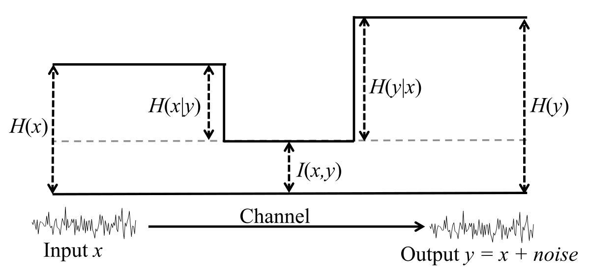
Mutual Information

Mutual information measures the mutual dependence between the two random variables, or equivalently, measures the information that these two random variables share. More specifically, it quantifies the “amount of information” obtained about one random variable through observing the other random variable.

Not limited to real-valued random variables and linear dependence like the correlation coefficient, mutual information is more general and determines how different the joint distribution \(P_{(X,Y)}(X,Y)\) is to the product of the marginal distributions \(P_{X}(X)P_{Y}(Y)\).

Definition

Given random variables $X,Y$ with sample spaces $\mathcal{X},\mathcal{Y}$ and possible outcomes $x\in\mathcal{X},y\in\mathcal{Y}$, the mutual information is defined as

\[\begin{align} I(X,Y) &:= D_{\text{KL}}(P_{(X,Y)} \parallel P_XP_Y) \\ &= E_P\bigg[\log \frac{P_{(X,Y)}(X,Y)}{P_X(X)P_Y(Y)} \bigg] \\ &= \sum_{y \in \mathcal Y} \sum_{x \in \mathcal X} { P_{(X,Y)}(x,y) \log{ \frac{P_{(X,Y)}(x,y)}{P_X(x)\,P_Y(y)} }}. \end{align}\]

Properties

Non-negativity: \(I(X,Y)\geq 0\) for any random variables \(X\) and \(Y\), and \(I(X,Y)=0\) and only if $X$ and $Y$ are independent.

Symmetry: \(I(X,Y) = I(Y,X)\) for any random variables \(X\) and \(Y\).

Relation to Conditional and Joint Entropy

\[\begin{align} I(X,Y) &= H(X) - H(X\mid Y) \\ &= H(Y) - H(Y \mid X) \\ &= H(X) + H(Y) - H(X,Y) \\ &= H(X,Y) - H(X\mid Y) - H(Y \mid X). \end{align}\]

References:

Wikipedia contributors. (2020, May 27). Entropy (information theory). In Wikipedia, The Free Encyclopedia. Retrieved May 31, 2020, from https://en.wikipedia.org/w/index.php?title=Entropy_(information_theory)&oldid=959218981.

Cover, T. M., & Thomas, J. A. (2012). Elements of information theory. John Wiley & Sons.

Wikipedia contributors. (2019, November 1). Joint entropy. In Wikipedia, The Free Encyclopedia. Retrieved May 31, 2020, from https://en.wikipedia.org/w/index.php?title=Joint_entropy&oldid=924098872.

Wikipedia contributors. (2020, May 24). Conditional entropy. In Wikipedia, The Free Encyclopedia. Retrieved May 31, 2020, from https://en.wikipedia.org/w/index.php?title=Conditional_entropy&oldid=958606256.

Wikipedia contributors. (2020, May 27). Kullback–Leibler divergence. In Wikipedia, The Free Encyclopedia. Retrieved May 31, 2020, from https://en.wikipedia.org/w/index.php?title=Kullback%E2%80%93Leibler_divergence&oldid=959167128.

Brownlee, J. (2019, December 19). A Gentle Introduction to Cross-Entropy for Machine Learning. Retrieved May 31, 2020, from https://machinelearningmastery.com/cross-entropy-for-machine-learning/.

Wikipedia contributors. (2020, May 27). Cross entropy. In Wikipedia, The Free Encyclopedia. Retrieved May 31, 2020, from https://en.wikipedia.org/w/index.php?title=Cross_entropy&oldid=959139954.

Wikipedia contributors. (2020, May 12). Mutual information. In Wikipedia, The Free Encyclopedia. Retrieved May 31, 2020, from https://en.wikipedia.org/w/index.php?title=Mutual_information&oldid=956303301.

Yao Xie. (2010, Dec 9). Entropy and mutual information. Retrieved May 31, 2020, from https://www2.isye.gatech.edu/~yxie77/ece587/Lecture2.pdf.