
Transfer learning is a research problem in machine learning that focuses on storing knowledge gained while solving one problem and applying it to a different but related problem. For example, knowledge gained while learning to recognize cars could apply when trying to recognize trucks.
A major assumption in many machine learning and data mining algorithms is that the training and future data must be in the same feature space and have the same distribution. However, in many real-world applications, this assumption may not hold. For example, we sometimes have a classification task in one domain of interest, but we only have sufficient training data in another domain of interest, where the latter data may be in a different feature space or follow a different data distribution. In such cases, knowledge transfer, if done successfully, would greatly improve the performance of learning by avoiding much expensive data labeling efforts.
Overview
Notations and Definitions
A domain \(\mathcal{D}\) consists of two components: a feature space \(\mathcal{X}\) and a marginal probability distribution \(P(X)\). The data instances \(x_1,\cdots,x_n \sim P(X)\) and \(x_1,\cdots,x_n \in \mathcal{X}\). Given a specific domain, \(\mathcal{D}=\{\mathcal{X},P(X)\}\), a task consists of two components: a label space \(\mathcal{Y}\) and an objective predictive function \(f(\cdot)\) (denoted by \(\mathcal{T} = \{\mathcal{Y}, f(·)\}\)), which is not observed but can be learned from the training data, which consist of pairs \(\{x_i,y_i\}\), where \(x_i \in \mathcal{X}\) and \(y_i \in \mathcal{Y}\). The function \(f(\cdot)\) can be used to predict the corresponding label, \(f(x)\), of a new instance \(x\). From a probabilistic viewpoint, \(f(x)\) can be written as \(P(y \mid x)\). In a classification problem, \(\mathcal{Y}\) is the set of all labels, which is True, False for a binary classification task, and \(y_i\) is “True” or “False”.
We consider the case where there is one source domain \(\mathcal{D}_S\) and one target domain \(\mathcal{D}_T\). More specifically, we denote the source domain data as \(\mathcal{D}_S = \{ (x_{S_1},y_{S_1}), \cdots, (x_{S_{n_S}},y_{S_{n_S}}) \}\), where \(x_{S_i} \in \mathcal{X}_S\) is the data instance and \(y_{S_1}\in\mathcal{Y}_S\) is the corresponding class label. Similarly, we denote the target domain data as \(\mathcal{D}_T = \{ (x_{T_1},y_{T_1}), \cdots, (x_{T_{n_T}},y_{T_{n_T}}) \}\). In most cases, \(0 \leq n_T \ll n_S\). We denote the source task as \(\mathcal{T}_S = \{\mathcal{Y}_S, f_S(·)\} = \{\mathcal{Y}_S, P\left(Y_{S} \mid X_{S}\right) \}\), and the target task as \(\mathcal{T}_T = \{\mathcal{Y}_T, f_T(·)\} = \{\mathcal{Y}_T, P\left(Y_{T} \mid X_{T}\right) \}\).
Definition. Transfer Learning. Given a source domain \(\mathcal{D}_S\) and source task \(\mathcal{T}_S\), a target domain \(\mathcal{D}_T\) and target task \(\mathcal{T}_T\), transfer learning aims to help improve the learning of the target predictive function \(f_T(·)\) in \(\mathcal{D}_T\) using the knowledge in \(\mathcal{D}_S\) and \(\mathcal{T}_S\), where \(\mathcal{D}_S \neq \mathcal{D}_T\), or \(\mathcal{T}_S \neq \mathcal{T}_T\).
When the target and source domains are the same, i.e. \(\mathcal{D}_{S}=\mathcal{D}_{T}\), and their learning tasks are the same, i.e., \(\mathcal{T}_{S}=\mathcal{T}_{T}\), the learning problem becomes a traditional machine learning problem.
The condition \(\mathcal{D}_{S} \neq \mathcal{D}_{T}\) implies that either \(\mathcal{X}_{S} \neq \mathcal{X}_{T}\) or \(P_{S}(X) \neq P_{T}(X)\). When the domains are different, i.e., \(\mathcal{D}_{S} \neq \mathcal{D}_{T}\), then either (1) the feature spaces between the domains are different, i.e. \(\mathcal{X}_{S} \neq \mathcal{X}_{T},\) or (2) the feature spaces between the domains are the same but the marginal probability distributions between domain data are different; i.e. \(P\left(X_{S}\right) \neq P\left(X_{T}\right),\) where \(X_{S_{i}} \in \mathcal{X}_{S}\) and \(X_{T_{i}} \in \mathcal{X}_{T}\). As an example, in our document classification example, case (1) corresponds to when the two sets of documents are described in different languages, and case (2) may correspond to when the source domain documents and the target domain documents focus on different topics.
Similarly, a task is defined as a pair \(\mathcal{T}=\{\mathcal{Y}, P(Y \mid X)\}\). Thus the condition \(\mathcal{T}_{S} \neq \mathcal{T}_{T}\) implies that either \(\mathcal{Y}_{S} \neq \mathcal{Y}_{T}\) or \(P\left(Y_{S} \mid X_{S}\right) \neq P\left(Y_{T} \mid X_{T}\right)\). Given specific domains \(\mathcal{D}_{S}\) and \(\mathcal{D}_{T},\) when the learning tasks \(\mathcal{T}_{S}\) and \(\mathcal{T}_{T}\) are different, then either (1) the label spaces between the domains are different, i.e. \(\mathcal{Y}_{S} \neq \mathcal{Y}_{T},\) or (2) the conditional probability distributions between the domains are different; i.e. \(P\left(Y_{S} \mid X_{S}\right) \neq P\left(Y_{T} \mid X_{T}\right),\) where \(Y_{S_{i}} \in \mathcal{Y}_{S}\) and \(Y_{T_{i}} \in \mathcal{Y}_{T} .\) In our document classification example, case (1) corresponds to the situation where source domain has binary document classes, whereas the target domain has ten classes to classify the documents to. Case (2) corresponds to the situation where the source and target documents are very unbalanced in terms of the user-defined classes.
Inductive Transfer Learning
Definition. Inductive Transfer Learning. Given a source domain \(\mathcal{D}_{S}\) and a learning task \(\mathcal{T}_{S}\), a target domain \(\mathcal{D}_{T}\) and a learning task \(\mathcal{T}_{T},\) inductive transfer learning aims to help improve the learning of the target predictive function \(f_{T}(\cdot)\) in \(\mathcal{D}_{T}\) using the knowledge in \(\mathcal{D}_{S}\) and \(\mathcal{T}_{S},\) where \(\mathcal{T}_{S} \neq \mathcal{T}_{T}\). In addition, a few labeled data in the target domain are required as the training data to induce the target predictive function.
Transductive Transfer Learning
Definition. Transductive Transfer Learning. Given a source domain \(\mathcal{D}_{S}\) and a corresponding learning task \(\mathcal{T}_{S},\) a target domain \(\mathcal{D}_{T}\) and a corresponding learning task \(\mathcal{T}_{T},\) transductive transfer learning aims to improve the learning of the target predictive function \(f_{T}(\cdot)\) in \(\mathcal{D}_{T}\) using the knowledge in \(\mathcal{D}_{S}\) and \(\mathcal{T}_{S},\) where \(\mathcal{D}_{S} \neq \mathcal{D}_{T}\) and \(\mathcal{T}_{S}=\mathcal{T}_{T} .\) In addition, some unlabeled target domain data must be available at training time.
Feature Extraction and Fine-Tuning in CNN
In practice, very few people train an entire network from scratch (with random initialization), because it is relatively rare to have a dataset of sufficint size. Instead, it is common to pretrain a network on a very large dataset (e.g. ImageNet, which contains \(1.2\) million images with \(1000\) categories), and then use the network either as an initialization or a fixed feature extractor for the task of interest.
In Convoluntional Neural Networks (CNNs), there are two commonly used types of transfer learning based on pretrained models: feature extraction and fine-tuning.
How Do They Work
In feature extraction, we start with a pretrained model and remove the final layer (usually a fully-connected layer and the outputs are the predicted class scores), and treat the rest of the CNN as a fixed feature extractor for the new dataset, then set the shape of the final layer and train this layer. We call these features CNN codes.
In fine-tuning, we not only replace and retrain the final layer, but to also fine-tune the weights of the pretrained network by continuing the backpropagation. It is possible to fine-tune all the layers of the CNN, or it’s possible to keep some of the earlier layers fixed (due to overfitting concerns) and only fine-tune the higher (latter) level layers. This is motivated by the observation that the earlier features (or activations) of a CNN contain more generic features (e.g. edge detectors or color blob detectors) that should be useful to many tasks, but later layers lattof the CNN becomes progressively more specific to the details of the classes contained in the original dataset. In case of ImageNet for example, which contains many dog breeds, a significant portion of the representational power of the CNN may be devoted to features that are specific to differentiating between dog breeds.
In general both transfer learning methods follow the same few steps:
-
Initialize the pretrained model;
-
Reshape the final layer (feature extraction) or layers (fine-tuning) to have the same number of outputs as the number of classes in the new dataset;
-
Define for the optimization algorithm which parameters we want to update during training;
-
Run the training step.
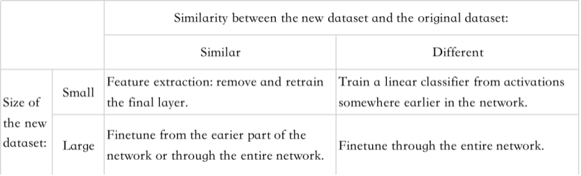
Which Type to Use
How do we decide what type of transfer learning we should perform on a new dataset? The two most important factors we need to consider are the size of the new dataset (small or big), and its similarity to the original dataset.
Keeping in mind that the CNN features are more generic in early layers and more original-dataset-specific in later layers. If our new dataset is large enough, we can fine-tune the pretrained model. If not, then we should not funetune the pretrained model due to overfitting concerns, and it may be better to use these data to train a linear classifier based on the CNN features. If the new dataset is similar to the original dataset, we expect higher (latter) level features in the pretrained model to be relevant to this new dataset as well, hence the feature extraction may be a good idea. However, if the two datasets are different, it might not be best to train a linear classifier form the top of the network, which contains more dataset-specific features. Instead, it might work better to train a linear classifier from CNN features somewhere earlier in the network.
Other Tips
Practical advice on learning rates: It’s common to use a smaller learning rate for CNN weights that are being fine-tuned, in comparison to the (randomly-initialized) weights for the new linear classifier that computes the class scores of your new dataset. This is because we expect that the CNN weights are relatively good, so we don’t wish to distort them too quickly and too much (especially while the new Linear Classifier above them is being trained from random initialization).
References:
Pan, Sinno Jialin, and Qiang Yang. “A survey on transfer learning.” IEEE Transactions on knowledge and data engineering 22.10 (2009): 1345-1359.
https://cs231n.github.io/transfer-learning/
https://pytorch.org/tutorials/beginner/fine-tuning_torchvision_models_tutorial.html