A linear regression model assumes that the regression function \(E(y_i \mid x_i)\) is linear in the inputs \(x_i^{(1)}, \cdots, x_i^{(p)}\). The linear regression model has the form \(\hat{y}_i = f(x_i) = \beta_0 + \underset{1 \times p}{\beta^T} \ \underset{p \times 1}{x_i} = \beta_0 + \sum_{j=1}^{p} \beta^{(j)} x_i^{(j)}\). If we set a \(1\) in the first position of the vector \(x_i\), then we can dismiss the intercept and the regression model can be written as \(\hat{y}_i = f(x_i) = \underset{1 \times p}{\beta^T} \ \underset{p \times 1}{x_i} = \sum_{j=1}^{p} \beta^{(j)} x_i^{(j)}\).

Let’s first suppose \(X\in\mathbb{R}^{n\times p}\) and \(y\in\mathbb{R}^n\), which means we have \(n\) observations and \(p\) features.

Ordinary Least Squares

The residual sum of squares:

\[\text{RSS}(\beta) = (y-X \beta)^T (y-X \beta) = \|y - X\beta \|^2_2 = \sum_{i=1}^{n}(y_i - \beta^T x_i)^2.\]

Closed-form solution for OLS (ordinary least squares) estimator

\[\hat{\beta} = \underset{\beta \in \mathbb{R}^p}{\text{argmin}} \ \text{RSS}(\beta) = (X^T X)^{-1} X^T y.\]

Hat matrix \(H = X (X^T X)^{-1} X^T\), which is positive semi-definite.

Assume \(\epsilon \sim N(0, \sigma^2)\), then \(\hat{\beta} \sim N(\beta, (X^TX)^{-1} \sigma^2)\).

More on The elements of Statistical Learning Page 47-49.

The Gauss-Markov Theorem: Least squares estimates of the parameter $\beta $ has the smallest variance among all linear unbiased estimates. This theorem means that the OLS estimator is BLUE (best linear unbiased estimator).

Derivation of OLS estimator: The first and second partial derivatives are

\[\frac{\partial \text{RSS}(\beta)}{\partial \beta} = -2 X^T (y-X \beta),\ \frac{\partial^2 \text{RSS}(\beta)}{\partial \beta \partial \beta^T} = 2 X^T X.\]

Assuming that \(X\) has full column rank, and hence \(X^TX\) is positive definite, we set the first derivative to zero and then we get the solution \(\hat{\beta} = (X^T X)^{-1} X^T y\).

We can also use gradient descent to find \(\hat{\beta}\). The gradient at \((t+1)\)-th iteration is \(\frac{\partial \text{RSS}(\beta_t)}{\partial \beta_t} = -2 X^T (y-X \beta_t)\).

Subset Selection

There are two reasons why we do variable subset selection:

• The first is prediction accuracy: the least squares estimates often have low bias but large variance. Prediction accuracy can sometimes be improved by shrinking or setting some coefficients to zero. By doing so we sacrifice a little bit of bias to reduce the variance of the predicted values, and hence may improve the overall prediction accuracy.
• The second reason is interpretation. With a large number of predictors, we often would like to determine a smaller subset that exhibit the strongest effects.

Forward-stepwise selection

Forward-stepwise starts with the intercept \(\bar{y}=\frac{1}{n}\sum_{i=1}^ny_i\), and then sequentially adds into the model the predictor that most improves the fit. It is a greedy algorithm, producing a nested sequence of models $M_0,M_1,…,M_P$, then we can select a single best model from among using cross-validated prediction error, $C_p$ (AIC), BIC or adjusted $R^2$.

The computation is $p(p-1)/2$. Advantages: computationally efficient, smaller variance as compared to best subset selection, but perhaps more bias; it can be used even when $p>n$. Disadvantages: errors made at the beginning cannot be corrected later.

Backward-stepwise selection

Backward-stepwise starts with the full model, and sequentially deletes the predictor that has the least impact on the fit.

Advantages: can throw out the “right” predictor by looking at the full model. Disadvantages: computationally inefficient (start with the full model), cannot work if $p>n$ .

Method	Optimality	Computation
Best subset	Best model guaranteed	\(2^p\)
Forward stepwise	No guarantee	\(p(p-1)/2\)
Backward stepwise	No guarantee	\(p(p-1)/2\)

There are several selection criteria like: \(C_p\), AIC, BIC, Adjusted \(R^2\).

Shrinkage Methods

Linear regression with L1-norm is LASSO and L2-norm is ridge regression.

Ridge regression:

\[\hat{\beta} = \underset{\beta \in \mathbb{R}^p}{\text{argmin}} \Big(\| y - X\beta \| ^2_2 + \lambda \| \beta \|^2_2 \Big) = (X^T X + \lambda I)^{-1} X^T y.\]

LASSO:

\[\hat{\beta} = \underset{\beta \in \mathbb{R}^p}{\text{argmin}} \Big( \|Y - X\beta \|^2_2 + \lambda \| \beta \|_1 \Big).\]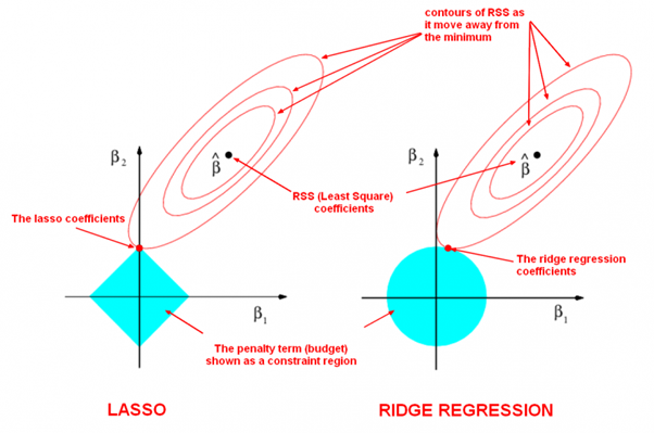

L1-norm shrinks some coefficients to $0$ and produces sparse coefficients, so it can be used to do feature selection. The sparsity makes the model more computationally efficient when doing prediction. L2-norm is differentiable so it has an analytical solution and can be calculated efficiently when training model.

Time Complexity

Suppose \(X\in\mathbb{R}^{n\times p}\) and \(y\in\mathbb{R}^n\), then the computational complexity of computing closed-form solution \((X^T X)^{-1} X^T y\) is \(O(pnp + p^3 + pn + p^2) = O(np^2+p^3)\). Here are the analyses:

1. The product \(X^TX\) takes \(O(pnp)\) time;
2. The inversion of \(X^TX\) takes \(O(p^3)\) time;
3. The product \(X^T y\) takes \(O(p n)\) time;
4. Finally, the multiplication of \((X^T X)^{-1}\) and \(X^T y\) takes \(O(p^2)\).

If we use gradient descent, at the \((t+1)\)-th iteration, computing the gradient \(\frac{\partial \text{RSS}(\beta_t)}{\partial \beta_t} = -2 X^T (y-X \beta_t)\) takes \(O(np+n+pn)=O(np)\) time. If we iterate \(M\) times, the time is \(O(Mnp)\). Here are the time complexity analyses for a iteration:

1. The product \(X\beta_t\) takes \(O(np)\) time;
2. The subtraction \(y-X \beta_t\) takes \(O(n)\) times;
3. The multiplication of \(-2X^T\) and \((y-X \beta_t)\) takes \(O(pn)\) time.

We may prefer gradient descent than computing the closed-form solution when \(p\) is very large.

We can also use the mini-batch gradient descent with batch size \(b\) (\(b < n\)), then the time of computing the gradient will be \(O(bp)\). However, in this case, we usually need more iterations than ordinary gradient descent, since the gradient is not that accurate. Note that if we set \(b=1\), it is stochastic gradient descent.