Neural Language Models

A neural LM (language model) usually has much higher predictive accuracy than an n-gram language model. Furthermore, neural language models underlie many of the models for tasks like machine translation, dialog, and language generation.

Compared to n-gram LMs, neural LMs don’t need smoothing, and they can handle much longer histories, and can generalize over contexts of similar words by using word embeddings.

However, neural net language models are strikingly slower to train than traditional language models, and so for many tasks an n-gram language model is still the right tool.

Embeddings

In neural language models, the prior context is represented by embeddings of the previous words. Representing the prior context as embeddings, rather than by exact words as used in n-gram language models, allows neural language models to generalize to unseen data much better than n-gram language models.

For example, suppose we’ve seen this sentence in training: “I have to make sure when I get home to feed the cat”, but we’ve never seen the word “dog” after the words “feed the”. In our test set we are trying to predict what comes after the prefix “I forgot when I got home to feed the”. An n-gram LM will predict “cat”, but not “dog”. But a neural LM, which can make use of the fact that “cat” and “dog” have similar embeddings, will be able to assign a reasonably high probability to “dog” as well as “cat”.

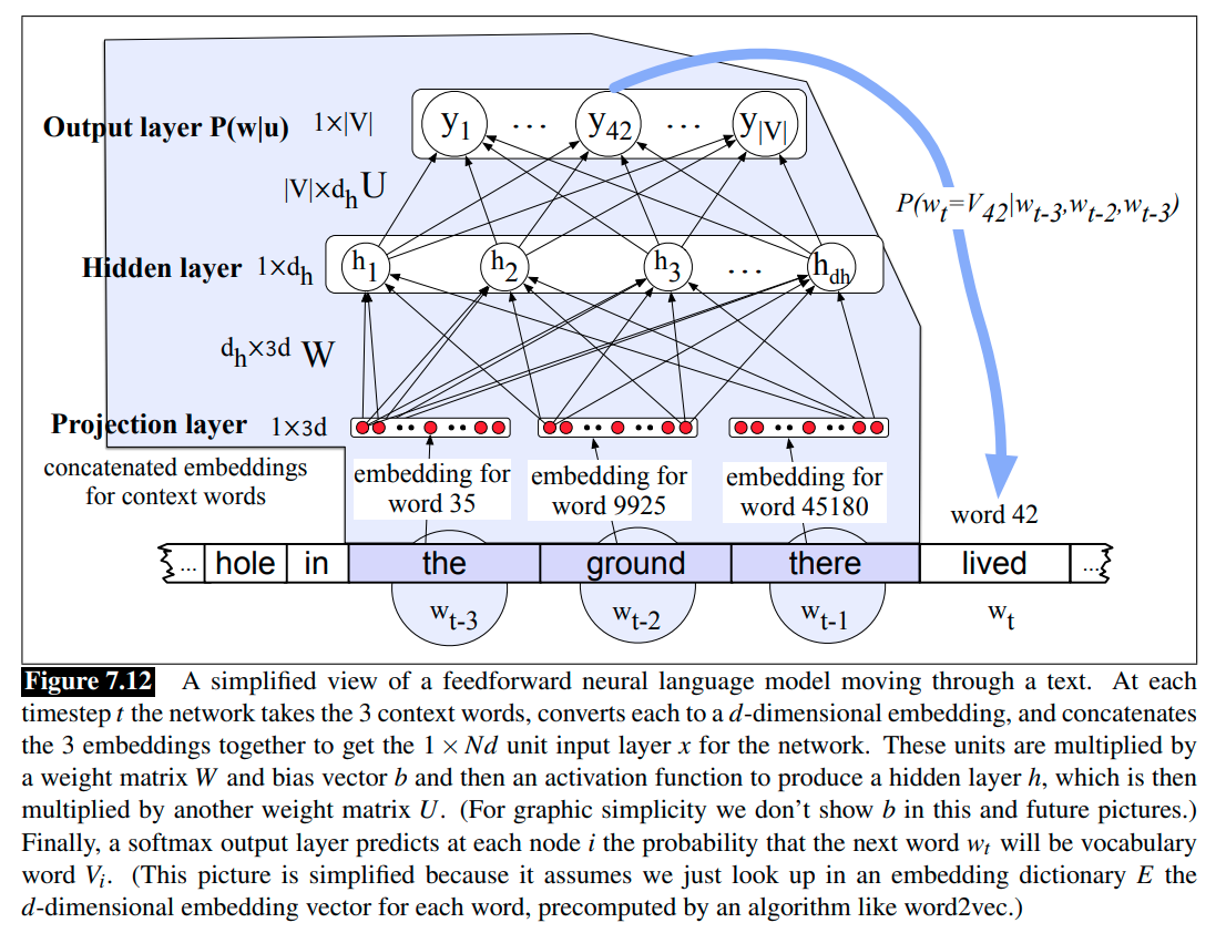
We can use the pre-trained word embeddings. As shown in the Figure 7.12, a feedforward neural LM with pre-trained embeddings as the inputs, and each embedding is of dimension \(d \times 1\).

However, often we’d like to learn the embeddings simultaneously with training the network. This is true when whatever task the network is designed for (sentiment classification, or translation, or parsing) places strong constraints on what makes a good representation.

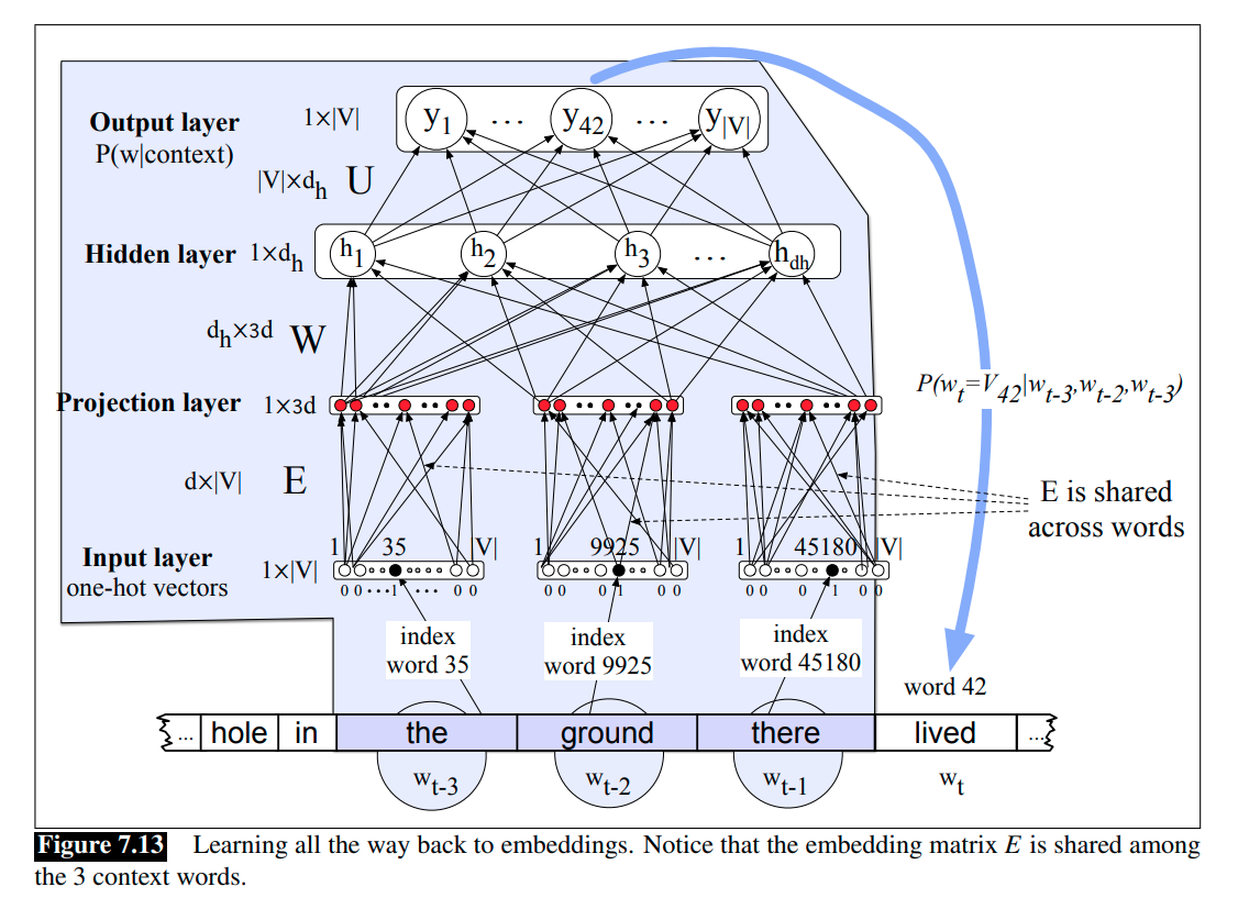
To do this, we’ll add an extra layer to the network, and propagate the error all the way back to the embedding vectors. For this to work at the input layer, instead of pre-trained embeddings, we’re going to represent each of the previous context words as a one-hot vector of length $\mid \mathcal{V} \mid$.

Sequence Processing with RNNs

The feedforward neural LMs operate by accepting fixed-sized windows of tokens as input; sequences longer than the window size are processed by sliding windows over the input making predictions as they go, with the end result being a sequence of predictions spanning the input. As shown in the Figure 7.12 and 7.13, we are predicting which word will come next given the window the ground there. Importantly, the decision made for one window has no impact on later decisions.

The sliding window approach is problematic for a number of reasons. One reason is that, it shares the primary weakness of Markov approaches in that it limits the context from which information can be extracted; anything outside the context window has no impact on the decision being made. This is an issue since there are many language tasks that require access to information that can be arbitrarily distant from the point at which processing is happening.

In a word, the feedforward neural LMs use the sliding window, which causes some problems. Recurrent neural networks (RNNs) are designed to overcome the weaknesses of sliding window approach, and RNNs allow us to handle variable length inputs without the use of fixed-sized windows.

Simple RNNs

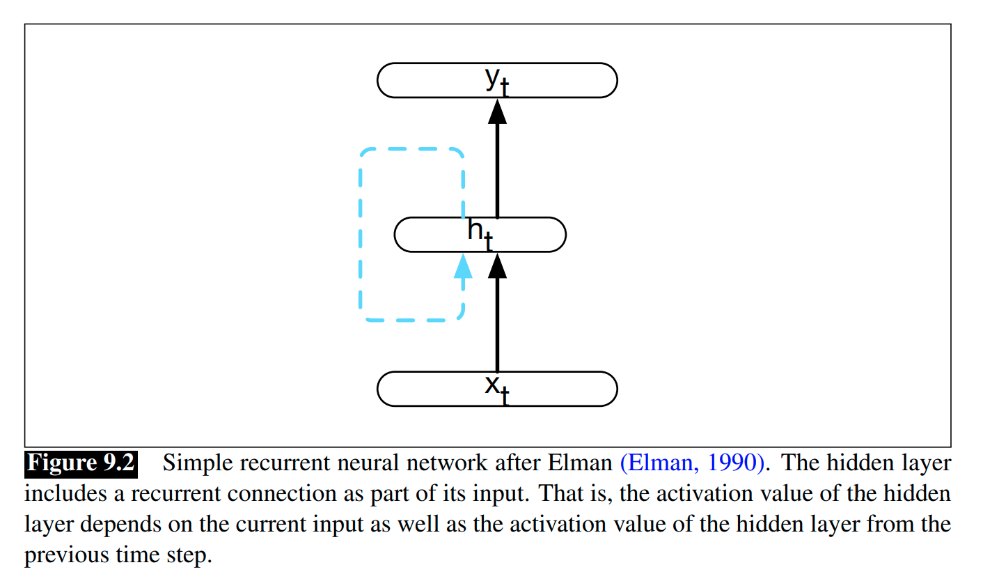
A recurrent neural network (RNN) is any network that contains a cycle within its network connections. That is, any network where the value of a unit is directly, or indirectly, dependent on earlier outputs as an input.

We first consider a class of recurrent networks referred to as Elman Networks or simple RNNs.

In a simple RNN, the hidden layer from the previous time-step provides a form of memory, or past context, that encodes earlier processing and informs the decisions to be made at later points in time.

Compared to non-recurrent architectures, we need another set of weights that connect the hidden layer from the previous time-step to the current hidden layer. These weights determine how the network should make use of memory (or past context) in calculating the output for the current input. As with the other weights in the network, these weights are trained via backpropagation.

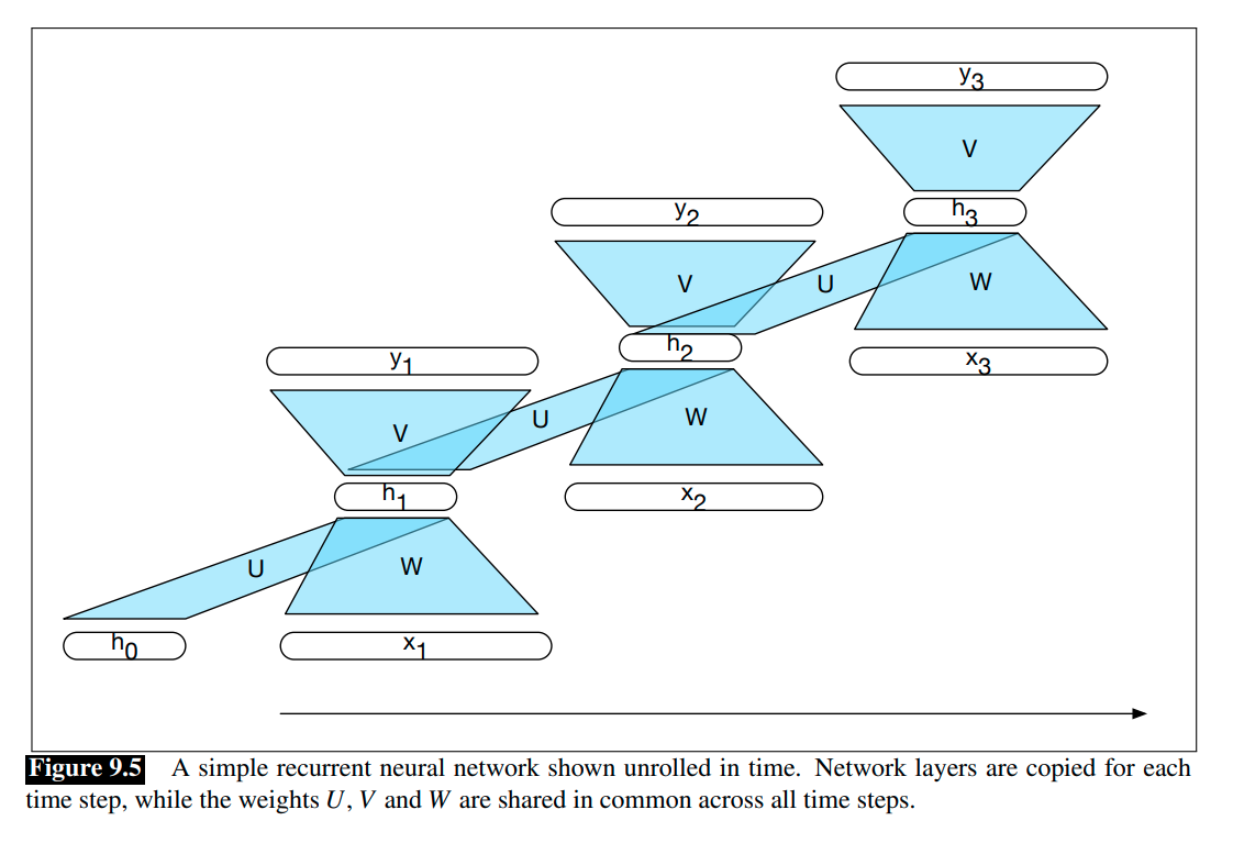
The following figures illustrate the structure of a simple RNN with one hidden layer.

Forward Inference in Simple RNNs

Forward inference in a RNN maps a sequence of inputs to a sequence of outputs. To compute an output $y_t$ for an input $x_t$, we need the activation value for the hidden layer $h_t$. To calculate this, we multiply the input $x_t$ with the weight matrix $W$, and the hidden layer from the previous time-step $h_{t-1}$ with the weight matrix $U$. We add these values together and pass them through a suitable activation function, $g(\cdot)$, to arrive at the activation value for the current hidden layer, $h_t$:

\[h_t = g(Uh_{t-1} + Wx_t).\]

Once we have the values for the hidden layer, we proceed with the usual computation to generate the output vector \(y_t\):

\[y_t = f(Vh_t).\]

In the commonly encountered case of soft classification, computing $y_t$ consists of a softmax computation that provides a normalized probability distribution over the possible output classes:

\[y_t = \text{Softmax}(Vh_t).\]

Suppose the parameters $U,V,W$ are known, with an input sequence $x=(x_1,x_3,\cdots,x_N)$, the forward inference, that gives us an output sequence \(y=(y_1,y_2,\cdots,y_N)\), in a simple RNN, can be expressed as

function FORWARD_RNN(x, network) returns output sequence y:
    h0 = 0 
    for t = 1 to LENGTH(x) do:
        ht = g(U * ht + W * xt) 
        yt = f(V * ht) 
    return y

Training Simple RNNs

As with other neural networks, we use a training set, a loss function, and backpropagation to obtain the gradients needed to adjust the weights in RNNs. We now have $3$ sets of weights to update: $W$, the weights from the input layer to the hidden layer, $U$, the weights from the previous hidden layer to the current hidden layer, and finally $V$, the weights from the hidden layer to the output layer.

Given an input sequence $x=(x_1,x_3,\cdots,x_N)$, the total loss (error) $L$ of an RNN is the sum of the loss at each time-step: \(L = \sum_{t=1}^N L_t = \sum_{t=1}^N \text{Loss}(\hat{y}_t, y_t)\).

Then the gradient of $W$ is

\[\frac{\partial L}{\partial W} = \frac{\partial \sum_{t=1}^N L_t}{\partial W} = \sum_{t=1}^N \frac{\partial L_t}{\partial W}.\]

The error for each time-step is computed through applying the chain rule differentiation:

\[\frac{\partial L_t}{\partial W} = \sum_{s=1}^t \frac{\partial L_t}{\partial y_t} \frac{\partial y_t}{\partial h_t} \frac{\partial h_t}{\partial h_s} \frac{\partial h_s}{\partial W}.\]

Also by the chain rule, each \(\frac{\partial h_t}{\partial h_s}\) is computed as

\[\frac{\partial h_t}{\partial h_s} = \frac{\partial h_t}{\partial h_{t-1}} \frac{\partial h_{t-1}}{\partial h_{t-2}} \cdots \frac{\partial h_{s+1}}{\partial h_s} = \prod_{r={s+1}}^{t} \frac{\partial h_r}{\partial h_{r-1}}.\]

Put these equations together and we have

\[\frac{\partial L}{\partial W} = \sum_{t=1}^N \sum_{s=1}^t \frac{\partial L_t}{\partial y_t} \frac{\partial y_t}{\partial h_t} \left( \prod_{r={s+1}}^{t} \frac{\partial h_r}{\partial h_{r-1}} \right) \frac{\partial h_s}{\partial W}.\]

The product form of these derivatives may lead to gradient explosion or gradient vanishing problem. Due to vanishing gradients, we don’t know whether there is dependency between different time steps in the data, or we just cannot capture the true dependency due to this issue.

To solve the problem of exploding gradients, Thomas Mikolov first introduced a simple heuristic solution that clips gradients to a small number whenever they reach a certain threshold, as shown below:

\[\begin{equation} \text{gradient} = \begin{cases} \frac{\partial L}{\partial W} & \text{ if } \| \frac{\partial L}{\partial W} \| \leq \text{threshold}, \\ \text{threshold} \cdot \frac{\frac{\partial L}{\partial W}}{\| \frac{\partial L}{\partial W} \|} & \text{ otherwise.} \end{cases} \end{equation}\]

To solve the problem of vanishing gradients, we introduce two techniques. The first technique is that instead of initializing $U$ randomly, start off from an identity matrix initialization. The second is to use the ReLU instead of the sigmoid function.

Stacked RNNs

In stacked RNNs, we use the entire sequence of outputs from one RNN as an input sequence to another one. Stacked RNNs consist of multiple networks, where The output of one RNN serves as the input to a subsequent RNN, as shown in Figure 9.10.

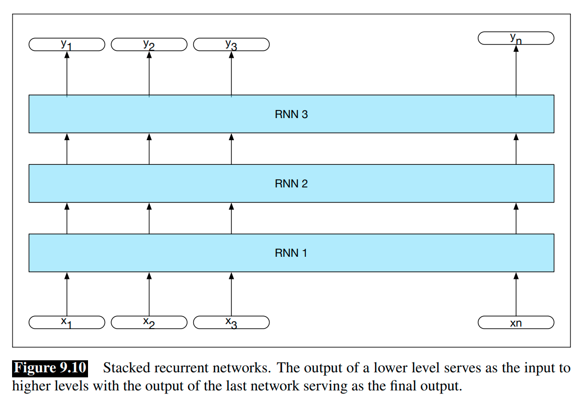
Stacked RNNs can usually outperform single-layer networks.

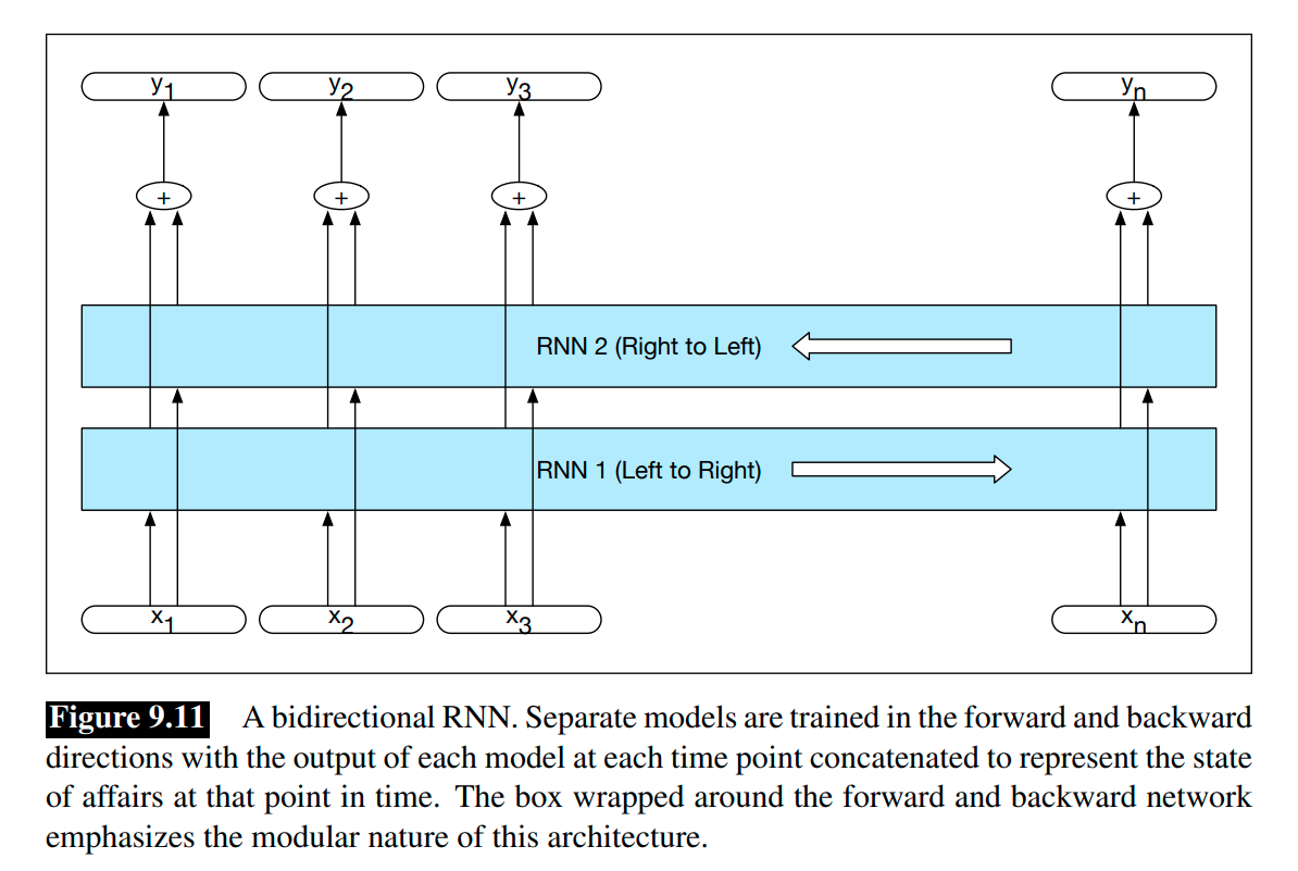
Bidirectional RNNs

We can train an backward RNN on an input sequence in reverse, using exactly the same kind of networks. Combining the forward and backward networks results in a bidirectional RNN.

A bidirectional RNN consists of two independent RNNs, one where the input is processed from the start to the end, and the other from the end to the start. We can use concatenation or simply element-wise addition or multiplication to combine the results of the two RNNs. The output at each step in time thus captures information to the left and to the right of the current input.

The bidirectional RNN for sequence labeling:

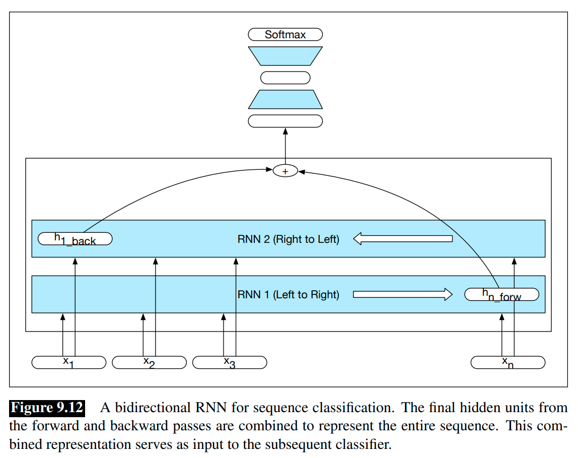
Bidirectional RNNs have proven to be quite effective for sequence classification, as shown in the Figure 9.12.

References:

Jurafsky, D., Martin, J. H. (2009). Speech and language processing: an introduction to natural language processing, computational linguistics, and speech recognition. Upper Saddle River, N.J.: Pearson Prentice Hall.

Mohammadi, M., Mundra, R., Socher, R., Wang, L., Kamath, A. (2019). CS224n: Natural Language Processing with Deep Learning, Lecture Notes: Part V, Language Models, RNN, GRU and LSTM. http://web.stanford.edu/class/cs224n/readings/cs224n-2019-notes05-LM_RNN.pdf.