
2 Pinhole cameras
As the aperture size decreases, the image gets sharper, but darker.
3 Cameras and lenses
In modern cameras, the above conflict between crispness and brightness is mitigated by using lenses.
A 3D point at further distance in front of the lens result in rays converge to a closer point behind the lens.
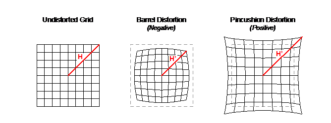
Because the paraxial refraction model approximates using the thin lens assumption, a number of aberrations can occur. The most common one is referred to as radial distortion, which causes the image magnification to decrease or increase as a function of the distance to the optical axis. We classify the radial distortion as pincushion distortion when the magnification increases and barrel distortion (e.g. fish-eye lenses) when the magnification decreases. Radial distortion is caused by the fact that different portions of the lens have differing focal lengths.
4 Going to digital image space
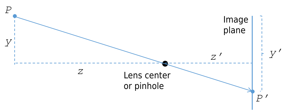
As discussed earlier, a point \(P\) in 3D space can be mapped (or projected) into a 2D point \(P'\) in the image plane \(\Pi'\). This \(\mathbb{R}^3 \to \mathbb{R}^2\) mapping is referred to as a projective transformation.
4.1 The Camera Matrix Model and Homogeneous Coordinates
4.1.1 Introduction to the Camera Matrix Mode
The camera matrix model describes a set of important parameters that affect how a world point \(P = (x,y,z)\) is mapped to image coordinates \(P' = (x',y')\).
\[P^{\prime}=\left[\begin{array}{l} x^{\prime} \\ y^{\prime} \end{array}\right]=\left[\begin{array}{l} k z' \frac{x}{z}+c_x \\ l z' \frac{y}{z}+c_y \end{array}\right]=\left[\begin{array}{l} \alpha \frac{x}{z}+c_x \\ \beta \frac{y}{z}+c_y \end{array}\right], \tag{4}\]where,
- \(x', y'\) are coordinates of a image point \(P'\) in digital image coordinates; they have units like “pixel”.
- \(z'\) are distance between image plane and lens center; it has unit like “cm”;
- \(x, y, z\) are coordinates of a world point \(P\) in world coordinates; they have units like “cm”;
- \(c_x, c_y\) are coordinates translation offsets; they have units like “pixel”; they are offsets between digital image coordinates (top left origin) and image plane coordinates (center origin); they equal to half digital image width and height.
- \(k, l\) are pixel density; they have units like “pixels per inch (ppi) or pixels per cm”; they may be different because the aspect ratio of a pixel is not guaranteed to be one; if they are equal, we often say that the camera has square pixels.
- \(\alpha = kz'\); \(\beta = lz'\).
4.1.2 Homogeneous Coordinates
From Equation (4), we see the projection \(P = (x,y,z) \to P' = (x',y')\) is not linear, as the operation divides \(z\). We can move to homogeneous coordinates to represent this projection as a matrix-vector product, which would be useful for future derivations.
To convert from Euclidean coordinate system to homogeneous coordinate system, we simply append a \(1\) in a new dimension. Any point \(P^{\prime}=\left(x^{\prime}, y^{\prime}\right)\) becomes \(\left(x^{\prime}, y^{\prime}, 1\right)\). Similarly, any point \(P=(x, y, z)\) becomes \((x, y, z, 1)\). When converting back from arbitrary homogeneous coordinates \(\left(v_1, \cdots, v_n, w\right)\), we get Euclidean coordinates \(\left(\frac{v_1}{w}, \cdots, \frac{v_n}{w}\right)\).
Using homogeneous coordinates, we can reformulate Equation (4) by a matrix vector relationship as
\[\begin{align} P^{\prime} &= \left[\begin{array}{c} x' \\ y' \\ 1 \end{array}\right] = \left[\begin{array}{c} \alpha \frac{x}{z}+c_x \\ \beta \frac{y}{z}+c_y \\ 1 \end{array}\right] = \left[\begin{array}{c} \alpha x+c_x z \\ \beta y+c_y z \\ z \end{array}\right] = \left[\begin{array}{cccc} \alpha & 0 & c_x & 0 \\ 0 & \beta & c_y & 0 \\ 0 & 0 & 1 & 0 \end{array}\right]\left[\begin{array}{c} x \\ y \\ z \\ 1 \end{array}\right] \\ &= \left[\begin{array}{cccc} \alpha & 0 & c_x & 0 \\ 0 & \beta & c_y & 0 \\ 0 & 0 & 1 & 0 \end{array}\right] P =\left[\begin{array}{ccc} \alpha & 0 & c_x \\ 0 & \beta & c_y \\ 0 & 0 & 1 \end{array}\right]\left[\begin{array}{ll} I & 0 \end{array}\right] P = K\left[\begin{array}{ll} I & 0 \end{array}\right] P. \end{align}\]4.1.3 Intrinsic Parameters
The following matrix \(K\) is the intrinsic parameters matrix without considering skewness and distortion:
\[K = \left[\begin{array}{ccc} \alpha & 0 & c_x \\ 0 & \beta & c_y \\ 0 & 0 & 1 \end{array}\right].\]As for skewness, the angle \(\theta\) between the two axes may be slightly larger or smaller than 90 degrees. The \(K\) accounting for skewness is
\[K = \left[\begin{array}{ccc} \alpha & -\alpha \cot \theta & c_x \\ 0 & \frac{\beta}{\sin \theta} & c_y \\ 0 & 0 & 1 \end{array}\right],\]Here \(K\) has 5 degrees of freedom:
- \(\alpha, \beta\) for scaling;
- \(c_x, c_y\) for translation offset;
- \(\theta\) for skewness.