The contents in this post are excerpted from the paper “Fast R-CNN” ¹, with a little bit modification, as my notes for this paper.

1. Introduction

Main contributions in brief: In this paper, the authors streamline the training process for R-CNN and SPP-net. The authors propose a single-stage training algorithm that jointly learns to classify object proposals and refine their spatial locations.

1.1 R-CNN and SPP-Net

Drawbacks of R-CNN and SPP-net:

• Training is a multi-stage pipeline that involves extracting features, fine-tuning a network with log loss, training SVMs, and finally fitting bounding-box regressors.
• Training is expensive in space and time. For SVM and bounding-box regressor training, features are extracted from each object proposal in each image and written to disk.
• As for R-CNN, it is slow because it performs a convolutional forward pass for each object proposal, without sharing computation.
• As for SPP-net, it is almost unable to finetune the convolutional layers that precede the SPP layer.

1.2 Contributions

Advantages of the proposed Fast R-CNN method over R-CNN and SPP-net:

• Faster to train and test;
• Higher detection quality (mAP);
• Training is single-stage, using a multi-task loss;
• Training can update all network layers;
• No disk storage is required for feature caching.

2. Fast R-CNN Architecture and Training

Figure 1 illustrates the Fast R-CNN architecture. A Fast R-CNN network takes as input an entire image and a set of object region proposals (proposed by methods like selective search).

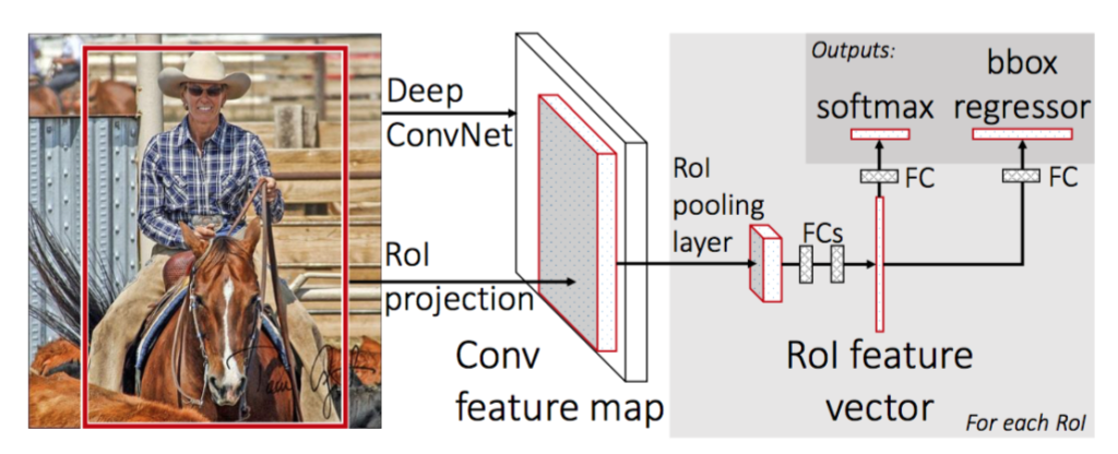
1. The network first processes the whole image with several convolutional and max pooling layers (denoted as “Deep ConvNet” in figure 1) to produce a conv feature map.
2. For each object region proposal (denoted as a red box on original image in figure 1), a region of interest (it is abbreviated as RoI, and it is a rectangular window into a conv feature map, and in figure 1 it is denoted as a gray cube with red borders in conv feature map) projected by RoI projection is then pooled into a fixed-size feature map (in figure 1 it is denoted as a gray cube with red borders pointed by “RoI pooling layer”) by RoI pooling layer, and then mapped to a fixed-length RoI feature vector by fully connected layers (FCs).
3. Each RoI feature vector is fed into a sequence of fully connected (FC) layers that finally branch into two sibling output layers: one that produces softmax probability estimates over \(K\) object classes plus a catch-all “background” class (\(K+1\) in total) and another layer that outputs 4 real-valued numbers (bounding-box regression offsets) for each of the \(K\) object classes (\(4K\) in total).

Fast R-CNN joint the (feature) extractor, classifier and regressor together in a unified framework.

Aside: What is feature map?

2.1 The RoI Pooling Layer

Given a RoI of size \(h \times w\) (unfixed), the RoI pooling layer is simply max pooling with approximate window size \(\frac{h}{H} \times \frac{w}{W}\), and the output is the RoI feature map of size \(H \times W\) (unfixed). The RoI pooling layer is simply the special-case of the SPP layer in which there is only one pyramid level.

2.3 Fine-Tuning for Detection

Training All Layers

SPP-net is almost unable to finetune the convolutional layers that precede the SPP layer. The root cause is that back-propagation through the SPP layer is highly inefficient when each training sample (i.e. RoI) comes from a different image, which is exactly how R-CNN and SPP-net networks are trained. For each RoI, the forward pass must process the entire corresponding receptive field, which is often very large (often the entire image), and thus the training inputs are large.

The authors propose a more efficient training method called hierarchical sampling that takes advantage of feature sharing during training. In Fast R-CNN training, stochastic gradient descent (SGD) mini-batches are sampled hierarchically, first by sampling \(N\) images and then by sampling \(\frac{R}{N}\) RoIs from each image. Critically, RoIs from the same image share computation and memory in the forward and backward passes. Making \(N\) small decreases mini-batch computation. For example, when using \(N = 2\) and \(R = 128\), the proposed training scheme is roughly \(64 \times\) faster than sampling one RoI from \(128\) different images (i.e., the R-CNN and SPPnet strategy). The experiment also shows that, with \(N = 2\) and \(R = 128\), the correlation between the RoIs in the same image does not leads to slow training convergence.

In addition to hierarchical sampling, Fast R-CNN uses a streamlined training process with one fine-tuning stage that jointly optimizes a softmax classifier and bounding-box regressors, rather than training a softmax classifier, SVMs, and regressors in three separate stages, as how R-CNN and SPP-net are trained.

Multi-Task Loss

A Fast R-CNN network has two sibling output layers. The first outputs a discrete probability distribution (per RoI), \(p=\left(p_{0}, \ldots, p_{K}\right)\), over \(K+1\) categories. As usual, \(p\) is computed by a softmax over the \(K+1\) outputs of a fully connected layer. The second sibling layer outputs bounding-box regression offsets, \(t^{k}=\left(t_{\mathrm{x}}^{k}, t_{\mathrm{y}}^{k}, t_{\mathrm{w}}^{k}, t_{\mathrm{h}}^{k}\right)\), for each of the \(K\) object classes, indexed by \(k\). We use the parameterization for \(t^{k}\) given in R-CNN, in which \(t^{k}\) specifies a scale-invariant translation and log-space height/width shift relative to an object proposal.

Each training RoI is labeled with a ground-truth class \(u\) and a ground-truth bounding-box regression target \(v\). We use a multi-task loss \(L\) on each labeled RoI to jointly train for classification and bounding-box regression:

\[L\left(p, u, t^{u}, v\right)=L_{\mathrm{cls}}(p, u)+\lambda\mathbb{1}_{\{u \geq 1\}} L_{\mathrm{loc}}\left(t^{u}, v\right),\]

in which \(L_{\mathrm{cls}}(p, u)=-\log p_{u}\) is log loss for true class \(u\).

The second task loss, \(L_{\text {loc }}\), is defined over a tuple of true bounding-box regression targets for class \(u, v=\) \(\left(v_{\mathrm{x}}, v_{\mathrm{y}}, v_{\mathrm{w}}, v_{\mathrm{h}}\right)\), and a predicted tuple \(t^{u}=\left(t_{\mathrm{x}}^{u}, t_{\mathrm{y}}^{u}, t_{\mathrm{w}}^{u}, t_{\mathrm{h}}^{u}\right)\), again for class \(u\). By convention the catch-all background class is labeled \(u=0\). For background RoIs there is no notion of a ground-truth bounding box and hence \(L_{\text {loc }}\) is ignored. For bounding-box regression, we use the loss

\(L_{\mathrm{loc}}\left(t^{u}, v\right)=\sum_{i \in\{\mathrm{x}, \mathrm{y}, \mathrm{w}, \mathrm{h}\}} \operatorname{smooth}_{L_{1}}\left(t_{i}^{u}-v_{i}\right),\) in which \(\operatorname{smooth}_{L_{1}}(x)=\left\{\begin{array}{ll} 0.5 x^{2} & \text { if }|x|<1 \\ |x|-0.5 & \text { otherwise } \end{array}\right.\)

is a robust \(L_{1}\) loss that is less sensitive to outliers than the \(L_{2}\) loss used in R-CNN and SPPnet. When the regression targets are unbounded, training with \(L_{2}\) loss can require careful tuning of learning rates in order to prevent exploding gradients. Eq. 3 eliminates this sensitivity.

The hyper-parameter \(\lambda\) in Eq. 1 controls the balance between the two task losses. We normalize the ground-truth regression targets \(v_{i}\) to have zero mean and unit variance. All experiments use \(\lambda=1\).

The experiments show that the single stage (multi-task) training used by Fast R-CNN performs better than multi stage training used by R-CNN and SPP-net.

3. Fast R-CNN Detection

3.1 Truncated SVD for Faster Detection

For detection the number of RoIs to process is large and nearly half of the forward pass time is spent computing the fully connected layers. Large fully connected layers are easily accelerated by compressing them with truncated SVD. This simple compression method gives good speedups when the number of RoIs is large.

Reference: