The contents in this post are excerpted from the paper “Faster R-CNN: Towards Real-Time Object Detection with Region Proposal Networks” ¹, with a little bit modification, as my notes for this paper.

Abstract

Advances like SPPnet and Fast R-CNN have reduced the running time of these detection networks, exposing region proposal computation as a bottleneck.

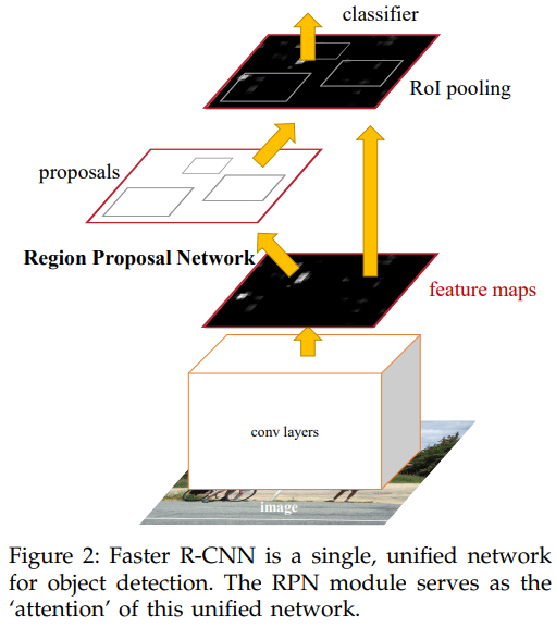
In this work, we introduce a Region Proposal Network (RPN) that shares full-image convolutional features with the detection network, thus enabling nearly cost-free region proposals. An RPN is a fully convolutional network that simultaneously predicts object bounds and objectness scores at each position. The RPN is trained end-to-end to generate high-quality region proposals, which are used by Fast R-CNN for detection. We further merge RPN and Fast R-CNN into a single network by sharing their convolutional features using the recently popular terminology of neural networks with “attention” mechanisms, the RPN component tells the unified network where to look.

1. Introduction

Selective Search, one of the most popular region proposal methods, is very slow.

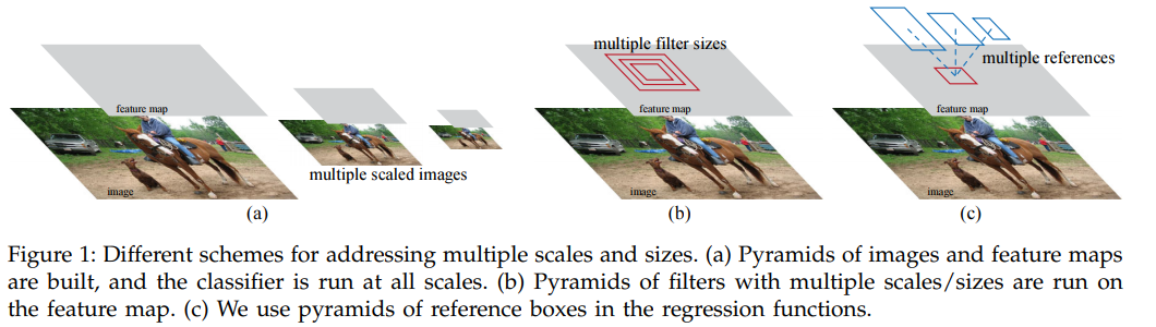
RPNs are designed to efficiently predict region proposals with a wide range of scales and aspect ratios. In contrast to prevalent methods like OverFeat, SPPnet and Fast R-CNN that use pyramids of images (Figure 1, a) or pyramids of filters (Figure 1, b), we introduce novel “anchor” boxes that serve as references at multiple scales and aspect ratios. Our scheme can be thought of as a pyramid of regression references (Figure 1, c), which avoids enumerating images or filters of multiple scales or aspect ratios. This model performs well when trained and tested using single-scale images and thus benefits running speed.

3. Faster R-CNN

Faster R-CNN, is composed of two modules: 1. RPN that proposes regions; 2. Fast R-CNN detector that uses the proposed regions. Both nets share a common set of convolutional layers. The RPN module tells the Fast R-CNN module where to look.

3.1 Region Proposal Networks

A Region Proposal Network (RPN) takes an image (of any size) as input and outputs a set of rectangular object proposals, each with an objectness score that measures membership to a set of object classes vs. background.

To generate region proposals, we slide a small network over the convolutional feature map output by the last shared convolutional layer. This small network takes as input an \(n \times n\) spatial window of the input convolutional feature map. Each sliding window is mapped to a lower-dimensional feature (256-d for ZF and 512-d for VGG, with ReLU following). This feature is fed into two sibling fully-connected layers—a box-regression layer (reg) and a box-classification layer (cls). We use \(n = 3\) in this paper.

3.1.1 Anchors

At each sliding-window location, we simultaneously predict multiple region proposals, where the number of maximum possible proposals for each location is denoted as \(k\). So the reg layer has \(4k\) outputs encoding the coordinates of \(k\) boxes, and the cls layer (two-class softmax layer) outputs \(2k\) scores that estimate probability of object or not object for each proposal (one may use logistic regression as the cls layer to produce \(k\) scores alternatively).

The \(k\) proposals are parameterized relative to \(k\) reference boxes, which we call anchors. An anchor is centered at the sliding window in question, and is associated with a scale and aspect ratio (Figure 3). By default we use \(3\) scales (box areas of \(128^2\), \(256^2\), and \(512^2\) pixels) and \(3\) aspect ratios (\(1:1\), \(1:2\), and \(2:1\)), yielding \(k = 9\) anchors at each sliding position. For a convolutional feature map of a size \(W \times H\) (typically \(\sim 2400\)), there are \(WHk\) anchors in total.

Translation-Invariant Anchors

An important property of our approach is that it is translation invariant, both in terms of the anchors and the functions that compute proposals relative to the anchors.

Multi-Scale Anchors as Regression References

Because of the multi-scale design based on anchors, we can simply use the convolutional features computed on a single-scale image, as is also done by the Fast R-CNN detector. The design of multi- scale anchors is a key component for sharing features without extra cost for addressing scales.

3.1.2 Loss Function

For training RPNs, we assign a binary class label (of being an object or not) to each anchor. We assign a positive label to two kinds of anchors: (i) the anchor/anchors with the highest Intersection-over-Union (IoU) overlap with a ground-truth box, or (ii) an anchor that has an IoU overlap higher than \(0.7\) with any ground-truth box. We assign a negative label to a non-positive anchor if its IoU ratio is lower than \(0.3\) for all ground-truth boxes. Anchors that are neither positive nor negative do not contribute to the training objective.

The loss function of RPN for an image is defined as:

\[L\left(\left\{p_{i}\right\},\left\{t_{i}\right\}\right)=\frac{1}{N_{c l s}} \sum_{i} L_{c l s}\left(p_{i}, p_{i}^{*}\right) + \lambda \frac{1}{N_{r e g}} \sum_{i} p_{i}^{*} L_{r e g}\left(t_{i}, t_{i}^{*}\right).\]

Here, \(i\) is the index of an anchor in a mini-batch and \(p_{i}\) is the predicted probability of anchor \(i\) being an object. The ground-truth label \(p_{i}^{*}\) is \(1\) if the anchor is positive, and is \(0\) if the anchor is negative. \(t_{i}\) is a vector representing the \(4\) parameterized coordinates of the predicted bounding box, and \(t_{i}^{*}\) is that of the ground-truth box associated with a positive anchor. The classification loss \(L_{c l s}\) is log loss over two classes (object vs. not object). For the regression loss, we use \(L_{\text {reg }}\left(t_{i}, t_{i}^{*}\right)=R\left(t_{i}-t_{i}^{*}\right)\) where \(R\) is the robust loss function (smooth \(\mathrm{L}_{1}\) ) defined in Fast R-CNN. The term \(p_{i}^{*} L_{\text {reg }}\) means the regression loss is activated only for positive anchors \(\left(p_{i}^{*}=1\right)\) and is disabled otherwise \(\left(p_{i}^{*}=0\right)\). The outputs of the \(c l s\) and reg layers consist of \(\left\{p_{i}\right\}\) and \(\left\{t_{i}\right\}\) respectively. The two terms are normalized by \(N_{c l s}\) and \(N_{r e g}\) and weighted by a balancing parameter \(\lambda\).

For bounding box regression, we adopt the parameterizations of the \(4\) coordinates as that in R-CNN:

\[\begin{aligned} t_{\mathrm{x}} &=\left(x-x_{\mathrm{a}}\right) / w_{\mathrm{a}}, \quad t_{\mathrm{y}}=\left(y-y_{\mathrm{a}}\right) / h_{\mathrm{a}}, \\ t_{\mathrm{w}} &=\log \left(w / w_{\mathrm{a}}\right), \quad t_{\mathrm{h}}=\log \left(h / h_{\mathrm{a}}\right), \\ t_{\mathrm{x}}^{*} &=\left(x^{*}-x_{\mathrm{a}}\right) / w_{\mathrm{a}}, \quad t_{\mathrm{y}}^{*}=\left(y^{*}-y_{\mathrm{a}}\right) / h_{\mathrm{a}}, \\ t_{\mathrm{w}}^{*} &=\log \left(w^{*} / w_{\mathrm{a}}\right), \quad t_{\mathrm{h}}^{*}=\log \left(h^{*} / h_{\mathrm{a}}\right), \end{aligned}\]

where \(x, y, w\), and \(h\) denote the box’s center coordinates and its width and height. Variables \(x, x_{\mathrm{a}}\), and \(x^{*}\) are for the predicted box, anchor box, and groundtruth box respectively (likewise for \(y, w, h)\). This can be thought of as bounding-box regression from an anchor box to a nearby ground-truth box.

In the previous RoI (Region of Interest) based methods like SPPnet and Fast R-CNN, bounding-box regression is performed on features pooled from arbitrarily sized RoIs, and the regression weights are shared by all region sizes. In our formulation, the features used for regression are of the same spatial size (\(3 \times 3\)) on the feature maps. To account for varying sizes, a set of \(k\) bounding-box regressors are learned. Each regressor is responsible for one scale and one aspect ratio, and the \(k\) regressors do not share weights.

3.1.3 Training RPNs

We follow the “image-centric” sampling strategy from Fast R-CNN to train this network.

3.2 Sharing Features for RPN and Fast R-CNN

Both RPN and Fast R-CNN, trained independently, will modify their convolutional layers in different ways. We use alternating training that allows for sharing convolutional layers between the two networks during training, rather than learning two separate networks.

In this paper, we adopt a 4-step alternating training. We initialize RPN and Fast R-CNN from pre-trained networks. We first train (fine-tune) RPN, then use the proposals from RPN to train (fine-tune) Fast R-CNN. At this point the two networks do not share convolutional layers. The tuned Fast R-CNN is then used to initialize RPN training, but we fix the shared convolutional layers and only fine-tune the layers unique to RPN. Now the two networks share convolutional layers. Finally, keeping the shared convolutional layers fixed, we fine-tune the unique layers of Fast R-CNN. As such, both networks share the same convolutional layers and form a unified network. A similar alternating training can be run for more iterations, but we have observed negligible improvements.

Reference: