The contents in this post are excerpted from the paper “Selective Search for Object Recognition” ¹, with a little bit modification, as my notes for this great paper.

Abstract

This paper addresses the problem of generating possible object locations for use in object recognition. The authors introduce selective search which combines the strength of both an exhaustive search and segmentation. Like segmentation, the selective search uses the image structure to guide our sampling process. Like exhaustive search, the selective search aims to capture all possible object locations.

1 Introduction

As for the problem of generating possible object locations for use in object recognition, there are two main approaches: segmentation and exhaustive search.

1.1 Segmentation

For a long time, objects were sought to be delineated before their identification. This gave rise to segmentation, which aims for a unique partitioning of the image through a generic algorithm.

Three problems for segmentation based methods:

1. Images are intrinsically hierarchical (e.g. a spoon in a bowl and the bowl on a table). This is most naturally addressed by using a hierarchical partitioning.
2. Individual visual features (e.g. colour, texture) cannot resolve the ambiguity of segmentation.
3. Regions with very different characteristics, such as a face over a sweater. Without prior recognition it is hard to decide that a face and a sweater are part of one object.

1.2 Exhaustive Search

Exhaustive search examines every location within the image as to not miss any potential object location. However, the search space is too huge and it has to be reduced by using restrictions like a regular grid, fixed scales, and fixed aspect ratios etc..

Rather then sampling locations blindly using an exhaustive search, a key question is: Can we steer the sampling by a data-driven analysis?

1.3 Inspired by These Two Approaches

In this paper, we aim to combine the best of the intuitions of segmentation and exhaustive search and propose a data-driven selective search. Inspired by bottom-up segmentation, we aim to exploit the structure of the image to generate object locations. Inspired by exhaustive search, we aim to capture all possible object locations. Therefore, instead of using a single sampling technique, we aim to diversify the sampling techniques to account for as many image conditions as possible.

Specifically, we use a data-driven grouping based strategy where we increase diversity by using a variety of complementary grouping criteria and a variety of complementary colour spaces with different invariance properties. The set of locations is obtained by combining the locations of these complementary partitionings.

Our goal is to generate a class-independent, data-driven, selective search strategy that generates a small set of high-quality object locations.

2 Related Work

2.1 Exhaustive Search

Sliding window techniques use a coarse search grid and fixed aspect ratios, using weak classifiers and economic image features such as HOG. For example, the HOG + SVM algorithm uses the HOG feature vector of a window as an input to the trained SVM to decide whether the window contains a (part of) target object.

Branch and bound technique uses the appearance model to guide the search.

2.2 Segmentation

2.3 Other Sampling Strategies

2.4 Novelty of Selective Search

• Instead of an exhaustive search, we use segmentation as selective search yielding a small set of class independent object locations.

• Instead of the segmentation methods that focus on the best segmentation algorithm, we use a variety of strategies to deal with as many image conditions as possible.

• Instead of learning an objectness measure on randomly sampled boxes , we use a bottom-up grouping procedure to generate good object locations.

3 Selective Search

Design considerations of selective search:

• Capture all scales (by hierarchical grouping).
• Diversification. We use a diverse set of strategies (colour, texture, size, and fill) to deal with all cases.
• Fast to compute. (it’s fast at that time)

3.1 Selective Search by Hierarchical Grouping

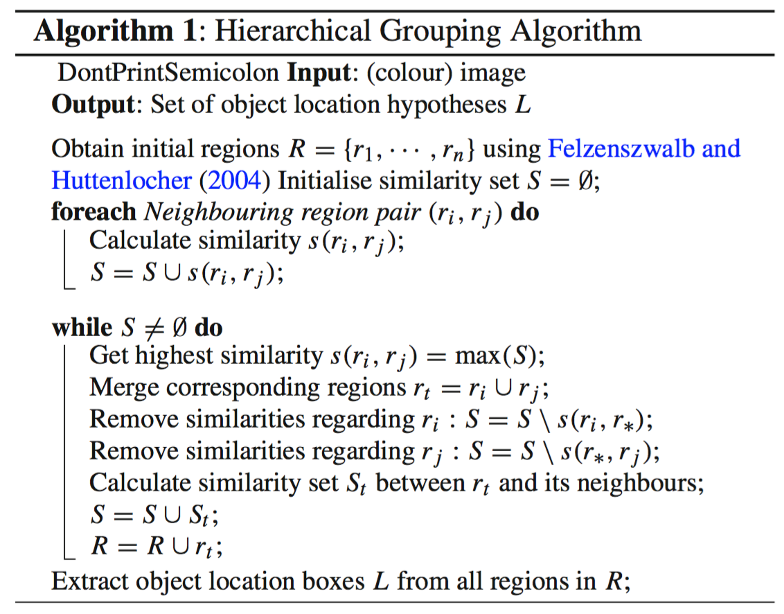
Our grouping procedure now works as follows. We first use “Felzenszwalb and Huttenlocher (2004)” to create initial regions. Then we use a greedy algorithm to iteratively group regions together: First the similarities between all neighbouring regions are calculated. The two most similar regions are grouped together, and new similarities are calculated between the resulting region and its neighbours. The process of grouping the most similar regions is repeated until the whole image becomes a single region. The general method is detailed in Algorithm 1.

For the similarity \(s(r_i, r_j)\) between region \(r_i\) and \(r_j\) we want a variety of complementary measures under the constraint that they are fast to compute. In effect, this means that the similarities should be based on features that can be propagated through the hierarchy, i.e. when merging region \(r_i\) and \(r_j\) into \(r_t\), the features of region \(r_t\) need to be calculated from the features of \(r_i\) and \(r_j\) without accessing the image pixels.

3.2 Diversification Strategies

We diversify our selective search by (1) using a variety of colour spaces with different invariance properties, (2) using different similarity measures \(s_{ij}\), and (3) varying our starting regions.

3.2.1 Complementary Colour Spaces

We want to account for different scene and lighting conditions. Therefore we perform our hierarchical grouping algorithm in a variety of colour spaces with a range of invariance properties (table 1): \(\text{RGB}\), intensity (grey-scale) \(I\), \(\text{Lab}\), \(\text{HSV}\), …

3.2.2 Complementary Similarity Measures

We define four complementary, fast-to-compute similarity measures (read the paper for detail):

• \(s_{\text{colour}}(r_i, r_j)\) measures colour similarity;
• \(s_{\text{texture}}(r_i, r_j)\) measures texture similarity;
• \(s_{\text{size}}(r_i, r_j)\) encourages small regions to merge early. It prevents a single region from gobbling up all other regions one by one.
• \(s_{\text{fill}}(r_i, r_j)\) measures how well region \(r_i\) and \(r_j\) fit into each other.

In this paper, our final similarity measure is a combination of the above four:

\[\begin{aligned} s\left(r_{i}, r_{j}\right) = &\ a_{1} s_{\text{colour}}\left(r_{i}, r_{j}\right)+a_{2} s_{\text {texture }}\left(r_{i}, r_{j}\right) \\ &+ a_{3} s_{\text{size}}\left(r_{i}, r_{j}\right)+a_{4} s_{\text{fill}}\left(r_{i}, r_{j}\right), \end{aligned}\]

where \(a_{i} \in\{0,1\}\) denotes if the similarity measure is used or not.

3.2.3 Complementary Starting Regions

Different starting regions are (already) obtained by varying the colour spaces, each which has different invariance properties. Additionally, we vary the threshold parameter \(k\) in “Felzenszwalb and Huttenlocher (2004)”.

3.3 Combining Locations

In this paper, we combine the object hypotheses of several variations of our hierarchical grouping algorithm. Ideally, we want to order the object hypotheses in such a way that the locations which are most likely to be an object come first.

We choose to order the combined object hypotheses set based on the order in which the hypotheses were generated in each individual grouping strategy. That means earlier grouped regions (lower hierarchy) are more possible to be an object. However, as we combine results from up to 80 different strategies, such order would too heavily emphasize large regions, because larger regions are more possible to appear in different grouping strategies. To prevent this, we include some randomness as follows.

Given a grouping strategy \(s\), let \(r_{h}^{s}\) be the region which is created at position \(h\) in the hierarchy, where \(h=1\) represents the top of the hierarchy (whose corresponding region covers the complete image). We now calculate the position value \(v_{h}^{s}\) as \(\text{RND} \times h\), where \(\text{RND}\) is a random number in range \([0,1]\). The final ranking is obtained by ordering the regions using \(v_{h}^{s}\).

Thus, the possibility score of a region \(r\) to be an object is

\[\begin{aligned} \text{score}(r) &= \sum_{s,h} \mathbb{1}(r_{h}^{s}=r) \cdot \text{score}(r_{h}^{s}) \\ &= \sum_{s,h} \mathbb{1}(r_{h}^{s}=r) \cdot v_{h}^{s} \\ &= \sum_{s,h} \mathbb{1}(r_{h}^{s}=r) \cdot \text{RND} \cdot h. \end{aligned}\]

Summary

To generate class-independent object locations, “selective search” initialize regions by “Felzenszwalb and Huttenlocher (2004)” and do hierarchical grouping (algorithm 1) with diversification strategies, then order the object hypotheses (regions, locations) by the possibility to be an object.

Reference: