Introduction

Goal of PCA

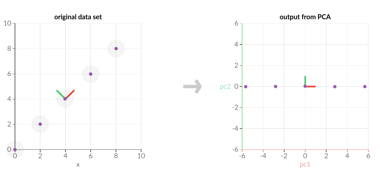
The goal of PCA (principal component analysis) is to reduce the dimension of the original data without losing too much information. In machine learning, we usually want to reduce the number of features of the original matrix \(\underset{n \times p}{X}\), that is, to find a matrix \(\underset{n \times d}{Z_d}\) that contains enough information of \(X\) but with \(d<p\), where \(n\) is the number of observations, \(p\) is the number of features and \(d\) is the number of features after PCA, which is also the number of components.

Centralization

The original data \(X=(x^{(1)}, \cdots ,x^{(p)})\) is of dimension \(n \times p\) with column vectors \(x^{(1)}, \cdots ,x^{(p)}\). Each column vector refers to a feature. At first, we centralize the original data by reducing the column mean:

Set \(x_i^{(j)} = x_i^{(j)} - \frac{1}{n} \sum_{i=1}^n x_i^{(j)}\) for all \(i=1,\cdots,n\) and all \(j=1,\cdots,p\).

After centralization, \(\sum_{i=1}^n x_i^{(j)} = 0\) or \(\bar{x}^{(j)}=0\).

Covariance Matrix

The \(i\)-th sample can be written as $x_i = (x_i^{(1)}, \cdots ,x_i^{(p)})^T$. We consider it as a random vector with dimension \(p\times 1\). The covariance matrix of \(x_i\) is

\[\begin{align} \text{Var}(x_i) &= \begin{pmatrix} \text{Var}(x_i^{(1)}) & \text{Cov}(x_i^{(1)}, x_i^{(2)}) & \cdots & \text{Cov}(x_i^{(1)}, x_i^{(p)}) \\ \text{Cov}(x_i^{(2)}, x_i^{(1)}) & \text{Var}(x_i^{(2)}) & \cdots & \text{Cov}(x_i^{(2)}, x_i^{(p)}) \\ \vdots & \vdots & \ddots & \vdots \\ \text{Cov}(x_i^{(p)}, x_i^{(1)}) & \text{Cov}(x_i^{(p)}, x_i^{(2)}) & \cdots & \text{Var}(x_i^{(p)}) \end{pmatrix} \\ &= \begin{pmatrix} E(x_i^{(1)} - Ex_i^{(1)})^2 & E[(x_i^{(1)} - Ex_i^{(1)}) (x_i^{(2)} - Ex_i^{(2)})] & \cdots & E[(x_i^{(1)} - Ex_i^{(1)}) (x_i^{(p)} - Ex_i^{(p)})] \\ E[(x_i^{(2)} - Ex_i^{(2)}) (x_i^{(1)} - Ex_i^{(1)})] & E(x_i^{(2)} - Ex_i^{(2)})^2 & \cdots & E[(x_i^{(2)} - Ex_i^{(2)}) (x_i^{(p)} - Ex_i^{(p)})] \\ \vdots & \vdots & \ddots & \vdots \\ E[(x_i^{(p)} - Ex_i^{(p)})(x_i^{(1)} - Ex_i^{(1)})] & E[(x_i^{(p)} - Ex_i^{(p)})(x_i^{(2)} - Ex_i^{(2)})] & \cdots & E(x_i^{(p)} - Ex_i^{(p)})^2 \end{pmatrix}. \end{align}\]

For arbitrary integer \(j, j'\) subject to \(1 \leq j, j' \leq p\) , we use \(\bar{x}^{(j)}\) to estimate \(E(x_i^{(j)})\), and \(\frac{1}{n-1} \sum_{i=1}^{n} (x_i^{(j)} - \bar{x}^{(j)}) (x_i^{(j')} - \bar{x}^{(j')})\) to estimate \(E[(x_i^{(j)} - Ex_i^{(j)})(x_i^{(j')} - Ex_i^{(j')})]\).

Since \(\bar{x}^{(j)}=0\) after centralization, we have the estimator of variance of arbitrary sample

\[\begin{align} S^2_x = \hat{\text{Var}}(x_i) &= \frac{1}{n-1} \begin{pmatrix} \sum_{i}{x_i^{(1)}}^2 & \sum_{i} x_i^{(1)} x_i^{(2)} & \cdots & \sum_{i} x_i^{(1)} x_i^{(p)} \\ \sum_{i}x_i^{(2)} x_i^{(1)} & \sum_{i} {x_i^{(2)}}^2 & \cdots & \sum_{i} x_i^{(2)} x_i^{(p)} \\ \vdots & \vdots & \ddots & \vdots \\ \sum_{i} x_i^{(p)} x_i^{(1)} & \sum_{i} x_i^{(p)} x_i^{(2)} & \cdots & \sum_{i} {x_i^{(p)}}^2 \end{pmatrix} \\ &= \frac{1}{n-1} \begin{pmatrix} {x^{(1)}}^T x^{(1)} & {x^{(1)}}^T x^{(2)} & \cdots & {x^{(1)}}^T x^{(p)} \\ {x^{(2)}}^T x^{(1)} & {x^{(2)}}^T x^{(2)} & \cdots & {x^{(2)}}^T x^{(p)} \\ \vdots & \vdots & \ddots & \vdots \\ {x^{(p)}}^T x^{(1)} & {x^{(p)}}^T x^{(2)} & \cdots & {x^{(p)}}^T x^{(p)} \\ \end{pmatrix} \\ &= \frac{1}{n-1} X^T X, \end{align}\]

which is the sample covariance matrix. Note that if \(X\) is not centered, then \(\frac{X^T X}{n-1}\) is not the sample covariance matrix.

Derive PCA through Orthogonal Transformation

Orthogonal Transformation

Suppose there is a orthogonal matrix \(\underset{p\times p}{W}\) with dimension \(p \times p\), then we transform \(X\) by \(W\) to get \(\underset{n\times p}{Z} = XW\). Denote \(\underset{n \times d}{Z_d}\) as the output of PCA, which is a sub-matrix of \(Z\). The rows of \(W\) are \(w_1^T, \cdots, w_p^T\), and the columns are \(w^{(1)}, \cdots, w^{(p)}\).

Orthogonal transformation to the centralized data \(X\) or \(x_i\):

\[\underset{n \times p}{X} \ \underset{p \times p}{W} = \underset{n \times p}{Z} \ \text{ or } \ \underset{n \times p}{X}\ \underset{p \times 1}{w^{(j)}} = \underset{n \times 1}{z^{(j)}} \ \text{ or } \ \underset{p \times p}{W} \ \underset{p \times 1}{x_i} = \underset{p \times 1}{z_i},\]

where \(z_i\) is the \(i\)-th observation after transformation with dimension \(p \times 1\) and \(z^{(j)}\) is the \(j\)-th principal component with dimension \(n \times 1\).

Similar to \(X\), the sample covariance matrix of \(z_i\) is \(\frac{1}{n-1} Z^T Z\).

Maximizing Variance

As we known, high variance means large amount of information.

The sample covariance matrix of \(z_i\) is \(S_z^2 = \hat{\text{Var}} (z_i) = \frac{1}{n-1} Z^T Z = \frac{1}{n-1} W^T X^T X W = W^T S_x^2 W.\)

The objective is to find \(W\) that maximize \(W^T S_x^2 W\):

\[W = \underset{W \in \mathbb{R}^{p \times p}}{\text{argmax }} W^T S_x^2 W, \\ \text{subject to } W^TW = I_p.\]

The sample variance of the \(j\)-th principal component \(z^{(j)}=Xw^{(j)}\) is

\[\hat{\text{Var}} (z_i^{(j)}) = \frac{1}{n-1} {z^{(j)}}^T z^{(j)} = \frac{1}{n-1} {w^{(j)}}^T X^T X w^{(j)} = {w^{(j)}}^T S^2_x w^{(j)}.\]

We find \(w^{(1)}, \cdots, w^{(p)}\) sequentially, then \(z^{(1)},z^{(2)},\cdots,z^{(p)}\) are 1st, 2nd, \(\cdots\), and \(p\)-th principal component. We can do this by gradient ascent, or more commonly by Lagrange multipliers, as shown below.

Optimization by Lagrange Multipliers

We find \(w^{(1)}, \cdots, w^{(p)}\) sequentially by using the method of Lagrange multipliers.

At first, we find \(w^{(1)}\) that maximize the sample variance of the first principal component

\[w^{(1)} = \underset{w^{(1)} \in \mathbb{R}^p}{\text{argmax }} \hat{\text{Var}} (z_i^{(1)}) = \underset{w^{(1)} \in \mathbb{R}^p}{\text{argmax }} {w^{(1)}}^T S^2_x w^{(1)}, \\ \text{ subject to } {w^{(1)}}^T w^{(1)} = 1.\]

Using the method of Lagrange multipliers, the Lagrangian function:

\[{\mathcal {L}} (w^{(1)}, \lambda_1) = {w^{(1)}}^T S^2_x w^{(1)} + \lambda ({w^{(1)}}^T w^{(1)} - 1).\]

Take derivatives of \({\mathcal {L}} (w^{(1)}, \lambda_1)\) with respect to \(w^{(1)}\) and \(\lambda_1\) then set to \(0\):

\[{\begin{cases} \frac{\partial {\mathcal {L}} (w^{(1)}, \lambda_1)} {\partial w^{(1)}} = S^2_x w^{(1)} - \lambda_1 w^{(1)} = 0, \\ \frac{\partial {\mathcal {L}} (w^{(1)}, \lambda_1)} {\partial \lambda_1} = {w^{(1)}}^T w^{(1)} - 1 = 0. \end{cases}}\]

Now we have \(S^2_x w^{(1)} = \lambda_1 w^{(1)}\), which means \(\lambda_1\) is a eigenvalue of \(S^2_x\) and \(w^{(1)}\) is the corresponding eigenvector.

In addition, \(\hat{\text{Var}} (z_i^{(1)}) = {w^{(1)}}^T S^2_x w^{(1)} = \lambda_1\), so we select the largest eigenvalue of \(S_x^2\) as \(\lambda_1\) since we want to maximize \(\hat{\text{Var}} (z_i^{(1)})\).

Then we find \(w^{(2)}\) that maximize the sample variance of the second principal component

\[w^{(2)} = \underset{w^{(2)} \in \mathbb{R}^p}{\text{argmax }} \hat{\text{Var}} (z_i^{(2)}) = \underset{w^{(2)} \in \mathbb{R}^p}{\text{argmax }} {w^{(2)}}^T S^2_x w^{(2)}, \\ \text{ subject to } {w^{(2)}}^T w^{(2)} = 1 \text{ and } {w^{(2)}}^T w^{(1)} = 0.\]

Lagrangian function:

\[{\mathcal {L}} (w^{(2)}, \lambda_2, \mu_2) = {w^{(2)}}^T S^2_x w^{(2)} + \lambda_2 ({w^{(2)}}^T w^{(2)} - 1) + \mu_2 ({w^{(2)}}^T w^{(1)} - 0).\]

Take derivatives of \({\mathcal {L}} (w^{(2)}, \lambda_2, \mu_2)\) with respect to \(w^{(2)}\), \(\lambda_2\) and \(\mu_2\), then set to \(0\). We have \(S^2_x w^{(2)} = \lambda_2 w^{(2)}\). \(\lambda_2\) is the second eigenvalue of \(S^2_x\) and \(w^{(2)}\) is the corresponding eigenvector.

Thus,

\[S_z^2 = W^T S_x^2 W = \begin{pmatrix} \lambda_1 & 0 & \cdots & 0 \\ 0 & \lambda_2 & \cdots & 0 \\ \vdots & \vdots & \ddots & \vdots \\ 0 & 0 & \cdots & \lambda_p \end{pmatrix},\]

where the columns of \(W\) are the eigenvectors of \(S_x^2\) and \(\lambda_1, \cdots \lambda_p\) are the corresponding eigenvalues.

\(\lambda_j\) is the sample variance of the \(j\)-th principal component.

\[{\lambda}_j = \hat{\text{Var}} (z^{(j)}) = \frac{ {z^{(j)}}^T z^{(j)}} {n-1} = {w^{(j)}}^T \frac{X^T X}{n-1} w^{(j)} = {w^{(j)}}^T S^2_x w^{(j)}.\]

Derive PCA through SVD

Singular Value Decomposition

Normal SVD: \(X = \underset{n\times n}{U}\ \underset{n\times p}{\Sigma}\ \underset{p\times p}{V^T}\).

Compact SVD: \(X = \underset{n\times r}{U}\ \underset{r \times r}{\Sigma}\ \underset{r \times p}{V^T}\), where \(r\) is the rank of \(X\); \(U\) and \(V\) are orthogonal matrices; \(\Sigma\) is a diagonal matrix with singular values \(\sigma_1, \cdots, \sigma_r\) on the diagonal. We prefer the compact SVD since it is more computationally effective.

Diagonalizing Covariance Matrix

We can also derive the result from the diagonalization of the covariance matrix.

Note that the diagonal entries of \(\frac{X^TX}{n-1}\) are the sample variance of each feature of \(X\), and the diagonal entries of \(\frac{Z^TZ}{n-1}\) are the sample variance of each principal components. Thus, we want to make \(\text{tr}(Z_d)\) as close as possible to \(\text{tr}(X)\). The larger \(\text{tr}(Z_d)\), the higher variance, and the larger information we can have in \(Z_d\).

An intuitive idea is to find a way to transform \(X^TX\) to a diagonal matrix \(Z^TZ\), then \(Z_d^T Z_d\) will be the sub-matrix of \(Z^TZ\) and contains the most highest \(d\) diagonal values of \(Z^TZ\). In this way, the information contained in \(Z_d\) will be largest.

SVD is a nice method to do this.

Suppose \(p=r\). Since \(U\) and \(V\) are both orthogonal, we have \(U^T=U^{-1}, V^T=V^{-1}\), then the compact SVD of \(X^TX\) is

\[X^TX = V \Sigma^T U^T \cdot U \Sigma V^T = V \Sigma^2 V^T.\]

It is also the eigenvalue decomposition of \(X^TX\). The columns of \(V\) are the eigenvectors of \(X^TX\) and the diagonal entries of \(\Sigma^2\) are the corresponding eigenvalues.

Now we have a diagonal matrix \(\Sigma^2\), then we set

\[Z^TZ = V^T X^T X V = \Sigma^2 = \begin{pmatrix} \sigma_1^2 & 0 & \cdots & 0 \\ 0 & \sigma_2^2 & \cdots & 0 \\ \vdots & \vdots & \ddots & \vdots \\ 0 & 0 & \cdots & \sigma_p^2 \end{pmatrix} .\]

Thus,

\[Z = XV.\]

The column vectors in \(V\) are the orthogonal basis vectors, which is the same as \(W\) and decide the directions of the principal components.

To get \(Z_d\), we select the \(d\) column vectors in \(V\) that corresponding to \(d\) largest eigenvalues \(\sigma_1^2, \cdots, \sigma_d^2\).

Low-Rank Approximation

Compact SVD of \(X\) can be decomposed as \(X = \underset{n\times r}{U}\ \underset{r \times r}{\Sigma}\ \underset{r \times p}{V^T} = \sum_{j=1}^r \sigma_j u_j v_j^T\), where \(u_1,\cdots,u_r\) and \(v_1,\cdots,v_r\) are column vectors of \(U\) and \(V\).

According to Eckart-Young-Mirsky theorem, we can approximate \(X\) by \(\sum_{j=1}^d \sigma_j u_j v_j^T\).

We have

\[XX^T = U \Sigma V^T \cdot V \Sigma^T U^T = U \Sigma^2 U^T, \\ Z_d Z_d^T = \underset{n \times d}{U_d} \ \underset{d \times d}{\Sigma_d^2} \ \underset{d \times n}{U_d^T}.\]

Therefore,

\[Z_d = U_d \Sigma_d.\]

Example, Tips and Summary

Example

\[X = \begin{pmatrix} 0 & 0 \\ 2 & 2 \\ 4 & 4 \\ 6 & 6 \\ 8 & 8 \end{pmatrix} - \begin{pmatrix} 4 & 4 \\ 4 & 4 \\ 4 & 4 \\ 4 & 4 \\ 4 & 4 \end{pmatrix} = \begin{pmatrix} -4 & -4 \\ -2 & -2 \\ 0 & 0 \\ 2 & 2 \\ 4 & 4 \end{pmatrix}.\] \[W = \begin{pmatrix} \frac{\sqrt{2}}{2} & \frac{-\sqrt{2}}{2} \\ \frac{\sqrt{2}}{2} & \frac{\sqrt{2}}{2} \end{pmatrix} , \ \ \ \ \ \ Z = XW = \begin{pmatrix} -4\sqrt{2} & 0 \\ -2\sqrt{2} & 0 \\ 0 & 0 \\ 2\sqrt{2} & 0 \\ 4\sqrt{2} & 0 \end{pmatrix}.\]

Tips

• The trace of a matrix equals to the sum of the eigenvalues. \(X^TX\) and \(XX^T\) have the same eigenvalues. \(\text{tr}(Z_d^T Z_d) = \text{tr}(Z_d Z_d^T) = \sum_{j=1}^{d} \sigma_j^2\), which equals to \(n-1\) times the sum of the sample variances of \(z^{(1)}, \cdots, z^{(d)}\). We also have \(\text{tr}(X^TX) = \text{tr}(Z^TZ) = \text{tr}(XX^T) = \text{tr}(ZZ^T) =\text{tr}(\Sigma^2) = \sum_{j=1}^p \sigma_j^2\), which also equals to \(n-1\) times the sum of the sample variances of \(x^{(1)}, \cdots, x^{(p)}\) or equivalently that of \(z^{(1)}, \cdots, z^{(p)}\).

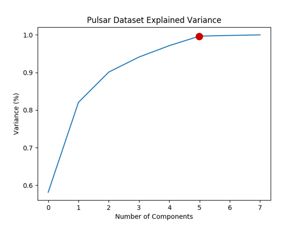
  Thus, the proportion of the information (variance) retained in the output \(Z_d\) is \(\text{tr}(\Sigma_d^2) / \text{tr}(\Sigma^2) = \sum_{j=1}^d \sigma_j^2 / \sum_{j=1}^p \sigma_j^2\).

• How to decide the number of components \(d\) ? We can plot the information (variance) proportion v.s. the number of components.

Summary

\[\begin{align*} \underset{n \times p}{X} = \underset{n\times p}{U}\ \underset{p \times p}{\Sigma}\ \underset{p \times p}{V^T} & \implies Z^TZ = V^T X^T X V = \Sigma^2 \implies \underset{n \times p}{Z} = XV \implies \underset{n \times d}{Z_d} = \underset{n \times p}{X}\ \underset{p \times d}{V_d}. \text{ (Cov matrix and ortho trans)} \\ \text{or} &\implies XX^T = U \Sigma^2 U^T \implies Z_d Z_d^T = \underset{n \times d}{U_d} \ \underset{d \times d}{\Sigma_d^2} \ \underset{d \times n}{U_d^T} \implies \underset{n \times d}{Z_d} = U_d \Sigma_d. \text{ (SVD low-rank approx)} \end{align*}\]

Sample covariance matrix of an arbitrary sample (denote as sample \(i\)) after PCA:

\[\begin{align*} \hat{\text{Var}}(z_i) &= S_z^2 = W^T S_x^2 W = \begin{pmatrix} \lambda_1 & 0 & \cdots & 0 \\ 0 & \lambda_2 & \cdots & 0 \\ \vdots & \vdots & \ddots & \vdots \\ 0 & 0 & \cdots & \lambda_p \end{pmatrix} \\ &= \frac{1}{n-1} Z^TZ = \frac{1}{n-1} V^T X^T X V = \frac{1}{n-1} \Sigma^2 = \frac{1}{n-1} \begin{pmatrix} \sigma_1^2 & 0 & \cdots & 0 \\ 0 & \sigma_2^2 & \cdots & 0 \\ \vdots & \vdots & \ddots & \vdots \\ 0 & 0 & \cdots & \sigma_p^2 \end{pmatrix} . \end{align*}\]

References:

Lecture notes from professor Min Xu.

张 洋. “PCA的数学原理.” CodingLabs, 22 June 2013.

Jonathan Hui, “Machine Learning - SVD and PCA.” Medium, 6 Mar 2019.