As for model fitting, with the increase in model complexity (i.e., the number of parameters), the Hough transform loses its effectiveness since the dimension of Hough space is too high; The RANdom SAmple Consensus (RANSAC) technique provides a computationally efficient means of fitting models in images.

Basic Idea

The RANSAC algorithm is used for estimating the parameters of models in images (i.e., model fitting). The basic idea behind RANSAC is to solve the fitting problem many times using randomly selected minimal subsets of the data and choosing the best performing fit. To achieve this, RANSAC tries to iteratively identify “inliers” and “outliers” in the data points that correspond to model we are trying to fit.

Applications

The RANSAC algorithm can be used to estimate parameters of different models; this is proven beneficial in image stitching, outlier detection, lane detection (linear model estimation), and stereo camera calculations.

The Algorithm

The RANSAC algorithm iteratively samples nominal subsets of the original data (e.g., 2 points for line estimation); the model is fitted to each sample, and the number of “inliers” corresponding to this fit is calculated. The points that are close to the fitted model (closer than a threshold, e.g., 2 standard deviation, or a pre-determined number of pixels) are considered “inliers”. The fitted model is considered good if a big fraction of the data is considered as “inliers” for that fit. After a good fit is found, the model is re-fitted using all the inliers. This process is repeated, and model estimates with a big enough fraction of inliers (e.g., bigger than a pre-specified threshold) are compared to choose the best-performing fit.

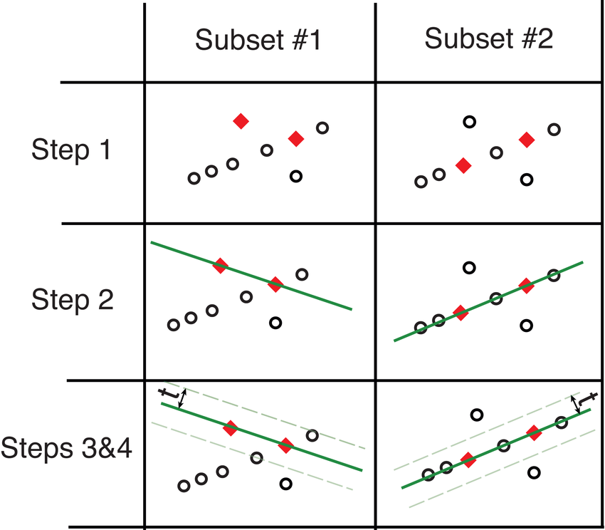
The major steps included in the RANSAC loop:

1. Randomly select a seed group of size \(n\) from data;

2. Perform parameter estimation using the selected seed group;

3. Identify the inliers (points close to the estimated model, e.g. distance is smalled than \(t\));

4. If there exists a sufficiently large number of inliers (larger than \(d\)), re-estimate the model using all inliers;

5. Repeat steps 1-4 and finally keep the estimate with most inliers and best fit.

Adaptive RANSAC

The RANSAC is a non-deterministic model fitting approach; this means that the number of samples need to be large enough to provide a high confidence estimate of parameters. The number of required samples depends on 1) the number of fitted parameters and 2) the amount of noise. More samples are needed for estimating bigger models and noisier data.

But how large is large enough? A large enough number of samples ($k$) need to be chosen such that a high confidence probability \(p\) (e.g. \(p=0.99\)) of at least one random sample is free from outliers is guaranteed:

\[p=1-(1-W^n)^k,\]

where $W$ and $n$ are respectively the fraction of inliers, and the number of points needed for model fitting.

Then the minimum number of samples is \(k=\frac{\log(1-p)}{\log(1-W^n)}\)

In practice, the fraction of inliers is usually unknown, and it can be estimated during the iterations of RANSAC. Thus the number of samples can also be determined adaptively during the iterations.

Algorithm. Adaptive procedure of RANSAC.

Set confidence probability \(p\) (e.g. \(p=0.99\));

Initialize sample count $c=0$, minimum number of samples $k=\infty$;

Initialize number of sampled points $NSP = 0$, number of inliers in the sampled points $NI = 0$;

While $c < k$:

  Choose a sample of size \(n\);

  Count the number of inliers in this sample \(\text{ni}\);

  $NSP \mathrel{+}= n$;

  $NI \mathrel{+}= \text{ni}$;

  Set fraction of inliers $W = \frac{NI}{NSP}$;

  Recompute $k$ from the new $W$ as $k=\frac{\log(1-p)}{\log(1-W^n)}$;

  $c \mathrel{+}= 1$;

End

Advantages, Limitations, and Considerations

Advantages of RANSAC:

• Simple implementation and wide application range in the model fitting domain;
• Computational efficiency;
• The sampling approach provides a better alternative to solving the problem for all possible combinations of features.

Disvantages:

• Only works well when you want to detect a single instance of a model (e.g. there is only a single line in image);
• Poor performance in highly noisy data (high ratio of outliers).

In some cases, it’d be more efficient to use the Hough transform instead of the RANSAC:

1. The number of parameters are small; for example, linear model estimation (2 parameters) can be achieved efficiently using Hough transform, while image stitching requires a more computationally frugal approach such as RANSAC.

2. If the noise ratio is high; as we saw earlier, increase in noise requires a more extensive sampling approach (higher number of samples), increasing computation cost. Increased noise reduces the chances of correct parameter estimation and the accuracy of inlier classification.

References: