
Here is a cheat sheet for big-O complexity of commonly used sorting algorithms:
| Algorithm | Best Time | Average Time | Worst Time | Space | Stable? | In-place? |
|---|---|---|---|---|---|---|
| Selection | $n^2$ | $n^2$ | $n^2$ | $1$ | ✓ | ✓ |
| Bubble | $n$ | $n^2$ | $n^2$ | $1$ | ✓ | ✓ |
| Insertion | $n$ | $n^2$ | $n^2$ | $1$ | ✓ | ✓ |
| Shell | $n\log_2 n$ | $n\log^2_2n$ | $n^2$ | $1$ | ✗ | ✓ |
| Tree | $n\log_2 n$ | $n\log_2 n$ | $n^2$ | $n$ | ✓ | ✗ |
| Heap | $n\log_2 n$ | $n\log_2 n$ | $n\log_2n$ | $1$ | ✗ | ✓ |
| Merge | $n\log_2 n$ | $n\log_2 n$ | $n\log_2n$ | $n$ | ✓ | ✗ |
| Quick | $n\log_2 n$ | $n\log_2 n$ | $n^2$ | $\log_2n$ or $n$ | ✗ | ✓ |
| Counting | $n+k$ | $ n+k $ | $n+k$ | $n+k$ | ✓ | ✗ |
| Radix | $l(n+c)$ | $l(n+c)$ | $l(n+c)$ | $n+c$ | ✓ | ✗ |
| Bucket | $n+b$ | $n+b$ | $n^2$ | $n+b$ | ✓ | ✗ |
Big-O asymptotic:
-
Definition: $T(N) = O(f (N))$ if there are positive constants $c$ and $n_0$ such that \(T(N) \le c \cdot f(N)\) for all \(N \geq n_0\).
-
Description: When $T(N) = O(f (N))$, we say that $T(N)$ is bounded above by $f(N)$ asymptotically (ignoring constant factors).
-
Checking: When $T(N) = O(f (N))$, check if \(\lim_{N\to\infty} \frac{T(N)}{f(N)} \approx \text{Constant}\).
Selection Sort and Bubble Sort
Selection Sort
The selection sort algorithm sorts an array by repeatedly finding the minimum element (considering ascending order) from unsorted part and putting it at the beginning of the previous unsorted part.
def selectionSort(arr):
    for i in range(len(arr)):
        # Find the minimum element in remaining unsorted array
        min_idx = i
        for j in range(i+1, len(arr)):
            if arr[min_idx] > arr[j]:
                min_idx = j
        # Swap the found minimum element with the first element of the remaining unsorted array
        arr[i], arr[min_idx] = arr[min_idx], arr[i]
Bubble Sort
Bubble sort works by repeatedly swapping the adjacent elements if they are in wrong order.
def bubbleSort(arr):
    for n in range(len(arr)-1, -1, -1):
        # arr[:n+1] are remaining unsorted
        swapped = False
        for j in range(0, n):
            # traverse the array from 0 to n, and swap if the element found is greater than the next element
            if arr[j] > arr[j+1] :
                arr[j], arr[j+1] = arr[j+1], arr[j]
                swapped = True
        if swapped == False:
            break
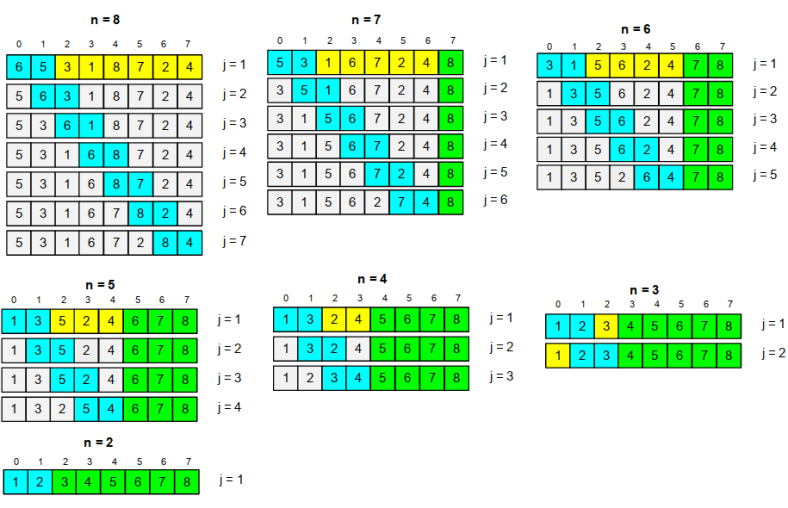
Note that \(O(n)\) is the best-case running time for bubble sort. By keeping track of the number of swaps it performs, if an array is already in sorted order, then bubble sort makes no swaps, the algorithm can terminate after one pass.
Insertion Sort and Shell Sort
Insertion Sort
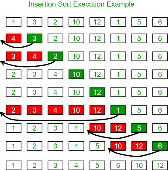
Insertion sort iterates, consuming one input element each repetition, and growing a sorted output list. At each iteration, insertion sort removes one element from the input data, finds the location it belongs within the sorted list, and inserts it there. It repeats until no input elements remain.
Python code:
def insertionSort(arr):
    for i in range(1, len(arr)):
        key = arr[i]
        # Move elements of arr[0..i-1], that are greater than key, to one position ahead their current position
        j = i-1
        while j >= 0 and key < arr[j] :
                arr[j + 1] = arr[j]
                j -= 1
        arr[j + 1] = key
Shell Sort
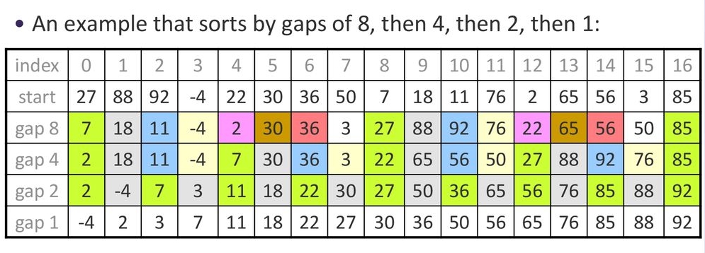
The shell sort, sometimes called the “diminishing increment sort”, improves on the insertion sort by breaking the original list into a number of smaller sublists, each of which is sorted using an insertion sort.
The unique way that these sublists are chosen is the key to the shell sort. Instead of breaking the list into sublists of contiguous items, the shell sort creates the sublists by an increment (sometimes called the gap).
There are two advantages of Shell Sort over Insertion Sort.
- When the swap occurs in a noncontiguous sublist, the swap moves the item over a greater distance within the overall array. Insertion Sort only moves the item one position at a time. This means that in Shell Sort, the items being swapped are more likely to be closer to its final position then Insertion Sort.
- Since the items are more likely to be closer to its final position, the array itself become partially sorted. Thus when the segment number equals one, and Shell Sort is performing basically the Insertion Sort, it will be able to work very fast, since Insertion Sort is fast when the array is almost in order.
Tree Sort and Heap Sort
They are both comparison based sorting techniques based on binary search trees and heaps.
Tree Sort
Tree sort builds a binary search tree (BST) for the elements and then traverses the tree in-order so that the elements come out in sorted order. It is faster for nearly sorted array.
Pseudo code:
def treeSort(arr):
	BST = buildBST(arr)
	return inOrderTraverse(BST)
Heap Sort
Heap sort first transforms the array into a heap (implemented as an array) in-place (time $O(n)$), then divides the array into a sorted and an unsorted region. We do the following steps iteratively (time $O(n\log_2n)$): 1. swap the first and last element in unsorted region; 2. shrink the unsorted region by merging the last element into the the sorted region. 3. re-heapify the shrunk unsorted region.
Pseudo code:
def heapSort(arr):
	buildHeap(arr) # in-place
	for i from len(arr)-1 to 1:
		swap(arr[0], arr[i])
		heapify(arr[:i])
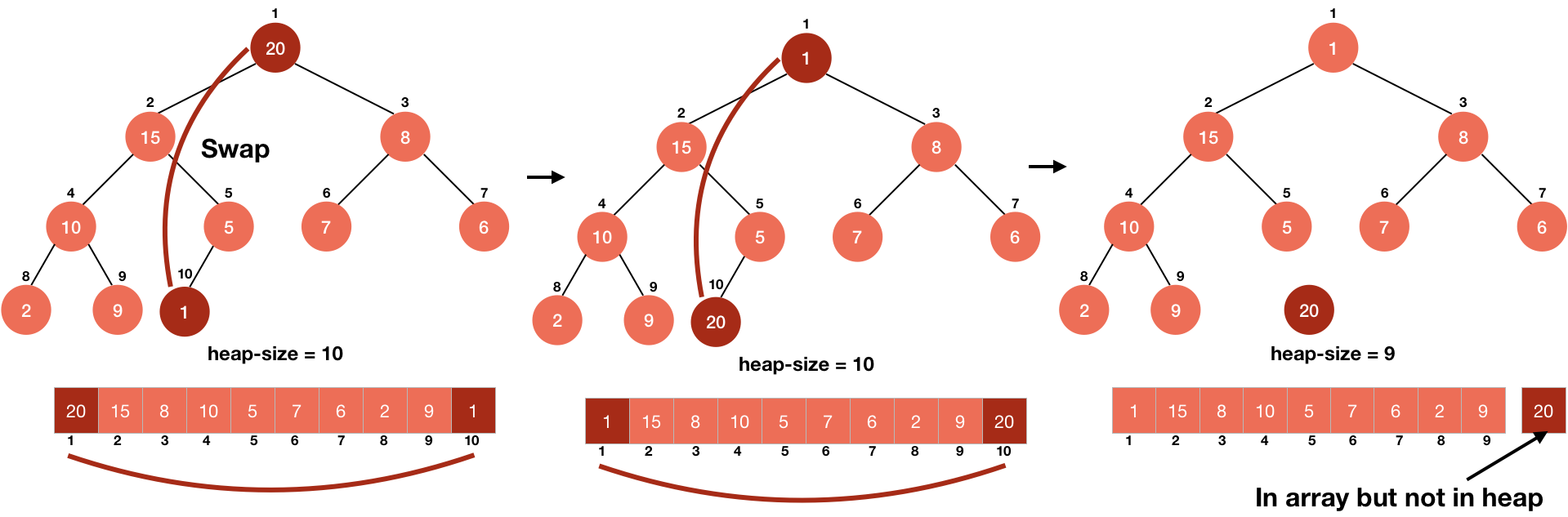
The left part (in heap) of the array is unsorted and the right part (not in heap) is sorted. We swap the first and last element in the unsorted array, then the last element is in the sorted array. Heap sort can be thought of as an improved selection sort.
Comparison
Heap sort is always preferable to tree sort in terms of either time or space:
- Time: The heap sort tends to be faster, because the heap is a balanced tree and its operations always are $O(\log_2n)$, in a determistic way, not on average. With BST, depending on the approach for balancing, insertion and deletion tend to take more time than the heap, no matter which balancing approach is used.
- Space: The heaps can be implemented as an array since they are always complete binary trees, but BSTs cannot because they are not guaranteed to be complete binary trees.
- Stability: Tree sort is stable, but heapsort is not because operations on the heap can change the relative order of equal items.
Merge Sort and Quick Sort
Both them employ the divide-and-conquer paradigm based on recursion. This paradigm breaks a problem into subproblems that are similar to the original problem, recursively solves the subproblems, and finally combines the solutions to the subproblems to solve the original problem.
Merge Sort
Divide the array into two sublists recursively and merge them.
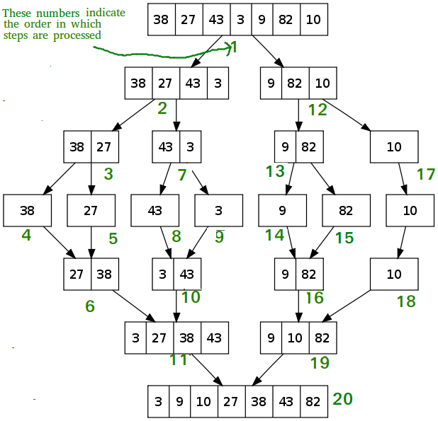
Space complexity analysis:
Suppose $n=16$, the space tree can be drawn as:
                     16                                 | 16
                    /  \
                   /    \
                  /      \
                 /        \
                8          8                            | 16
               / \        / \
              /   \      /   \
             4     4    4     4                         | 16
            / \   / \  / \   / \
           2   2 2   2 .......  2                       | 16
          / \  /\  ............ /\
         1  1  1 1 ............ 1 1                     | 16
The largest memory in recursion is:
                       16
                      /
                     8
                    /
                   4
                  /
                 2
               / \
              1   1
Thus, the space complexity is $O(3n)=O(n)$.
Merge Sort on Linked List
# Definition for singly-linked list.
class ListNode(object):
    def __init__(self, x):
        self.val = x
        self.next = None

class Solution:
    def sortList(self, head: ListNode) -> ListNode:
        if not head or not head.next:
            return head
        slow, fast = head, head.next
        while fast and fast.next:
            slow = slow.next
            fast = fast.next.next
        second = slow.next
        slow.next = None
        l = self.sortList(head)
        r = self.sortList(second)
        return self.merge(l, r)

    def merge(self, l: ListNode, r: ListNode) -> ListNode:
        if not l or not r:
            return l or r
        if l.val > r.val:
            l, r = r, l
        # get the return node "head"
        head = pre = l
        l = l.next
        while l and r:
            if l.val < r.val:
                l = l.next
            else:
                nxt = pre.next
                pre.next = r
                tmp = r.next
                r.next = nxt
                r = tmp
            pre = pre.next
        # l and r at least one is None
        pre.next = l or r
        return head
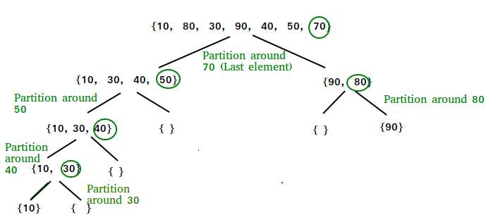
Quick Sort
Recursively pick an element as pivot and partition the other elements by comparing them with the picked pivot.
Best case: In the best case, each time we perform a partition we divide the list into two nearly equal pieces. The depth of the recurrence tree is $\log_2n$. The time in each level of the recurrence tree is $O(n)$. Thus, in the best case, the time complexity is $O(n\log_2n)$ and the space complexity is $O(\log_2n)$.
Worst case: If the leftmost (or rightmost) element is chosen as pivot, the worst occurs when the array is already sorted in order or reverse order (a special case is that all elements are same). At this situation, every element will be a pivot, thus the time is \((n-1) + (n-2) + \cdots + 1 = \frac{n(n-1)}{2} = O(n^2)\), and the recurrence tree will be a right or left skewed tree thus the space is $O(n)$. The problem can be easily solved by choosing a random or middle index for the pivot. However, the worst case can still occurs when all elements are same.
Comparisons between Heap, Merge and Quick Sort
Heap sort is the slowest. Heap sort may make more comparisons than optimal. Each siftUp operation makes two comparisons per level, so the comparison bound is approximately \(2n\log_2 n\). Heap Sort is more memory efficient and also in place. Merge sort is slightly faster than the heap sort for larger sets.
Quick sort is usually faster than most other $O(n\log_2n)$ comparison based algorithms in practice. The reasons are:
- Cache efficiency. Quick sort changes the array in-place, and it linearly scans the input and linearly partitions the input. Thus, it applies the principle of locality of reference. Cache benefits from multiple accesses to the same place in the memory, since only the first access needs to be actually taken from the memory, and the rest of the accesses are taken from cache, which is much faster than the access to memory. For heap sort, it needs to swap the elements that are usually not close to each other. If $n$ is large, the cache cannot store the heap array, thus we need to access the memory (RAM) frequently. Merge sort needs much more RAM accesses, since every accessory array you create is accessing the RAM again. Trees are even worse, since it is not in-place and two sequential accesses in a tree are not likely to be close to each other.
- No unnecessary elements swaps. Swap is time consuming. With quick sort we don’t swap what is already ordered. The main competitors of quick sort are merge sort and heap sort. With heap sort, which is also in-place, even if all of your data is already ordered, we are going to swap all elements to order the array. With merge sort, which is not in-place, it’s even worse, since you are going to write all elements in another array and write it back in the original one, even if data is already ordered. However, it doesn’t mean heap sort is always faster than merge sort.
Comparison between merge sort and quick sort
In-place Quick Sort on Array in Python
def partition(arr: list, start: int, end: int) -> int:
    """returns the partition index"""
    j = start
    for i in range(start, end):
        # use arr[end] as pivot
        if arr[i] < arr[end]:
            # swap to make the elements in arr[:j] be smaller than pivot
            arr[j], arr[i] = arr[i], arr[j]
            j += 1
    arr[j], arr[end] = arr[end], arr[j]
    # now the elements in arr[:j] are smaller than arr[j],
    # and the elements in arr[j+1:] are larger than arr[j]
    return j

# another partition method
def partition(arr: list, start: int, end: int) -> int:
    """returns the partition index"""
    i, j = start, end # left index i, and right index j
    # use arr[end] as pivot
    while i < j:
        # find i that makes arr[i] >= pivot
        while i < j and arr[i] < arr[end]:
            i += 1
        # find j that makes arr[j] < pivot
        while i < j and arr[j] >= arr[end]:
            j -= 1
        # swap left large element arr[i] and right small element arr[j]
        arr[i], arr[j] = arr[j], arr[i]
    # now i == j, swap pivot and arr[j]
    arr[end], arr[j] = arr[j], arr[end]
    # now the elements in arr[:j] are < arr[j],
    # and the elements in arr[j+1:] are >= arr[j]
    return j
def quicksort(arr: list) -> list:
    """in-place quicksort function"""

    def helper(arr: list, start: int, end: int) -> None:
        """recursive helper"""
        if start >= end: return None
        j = partition(arr, start, end) # partition index
        helper(arr, start, j-1) # sort the left part arr[:j]
        helper(arr, j+1, end) # sort the right part arr[j+1:]

    helper(arr, 0, len(arr)-1)
In-place Quick Sort on Linked List in Python
# Definition for singly-linked list.
class ListNode(object):
    def __init__(self, x):
        self.val = x
        self.next = None

class Solution(object):
    def sortList(self, node):
        if not node or not node.next:
            return node
        pivot = node
        node = node.next
        pivot.next = None
        left = dummyLeft = ListNode(None)
        right = dummyRight = ListNode(None)

        while node:
            if node.val < pivot.val:
                left.next = node
                left = left.next
            else:
                right.next = node
                right = right.next
            node = node.next
        left.next = None
        right.next = None

        headLeft = self.sortList(dummyLeft.next)

        if not headLeft:
            headLeft = pivot
        else:
            tailLeft = headLeft
            while tailLeft.next:
                tailLeft = tailLeft.next
            tailLeft.next = pivot
        pivot.next = self.sortList(dummyRight.next)

        return headLeft
Non-Comparison Sort Algorithm
Counting Sort
Counting sort is usually used for sorting integers or characters. It is based on keys between a specific range. It works by counting the number of objects having distinct key values (kind of hashing). Then doing some arithmetic to calculate the position of each object in the output sequence.
Suppose the elements are in range from $1$ to $k$, thus there are $k$ keys.
# Python code for counting sort.
def countingSort(input: list, k: int) -> list:
    count = k * [0]
    for x in input:
        count[key(x)] += 1
    for j in range(1, k):
        count[j] += count[j-1]
    output = len(input) * [None]
    for x in input[::-1]:
        count[key(x)] -= 1
        output[count[key(x)]] = x
    return output
Time complexity of initializing the counting array of size $k$ is $O(k)$, and that of counting all elements is $O(n)$. Thus the time complexity of counting sort is $O(n+k)$. Space complexity is $O(k)$ since the size of the counting array is $k$.
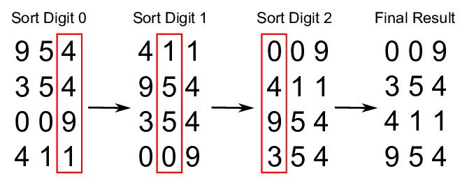
Radix Sort
Counting sort is a linear time sorting algorithm that sort in $O(n+k)$ time when elements are in range from $1$ to $k$. However, if the elements are in a big range, for example, from $1$ to $n^2$, then $k=O(n^2)$, we cannot use counting sort because it will take $O(n^2)$ which is worse than comparison based sorting algorithms.
In this case, radix sort can sort such an array in linear time. The idea of Radix sort is to do digit by digit sort starting from least significant digit to most significant digit. Radix sort uses counting sort as a subroutine to sort.
Suppose there are $l$ digits(or characters) in each input integer(or string), and there are $c$ different digits(or characters), for example, $c=10$ for digits and $c=26$ for characters. Note that $c$ is the size of the count array in each counting sort of each pass, also $k=O(c^l)$.
In radix sort, we perform counting sort for $l$ passes, and each counting sort takes $O(n+c)$ time, thus the time complexity of radix sort is $O(l(n+c))$. The space complexity also comes from counting sort, which requires $O(n+c)$ space.
# use the bucket sort internally.
def radixSort(self, nums: list) -> int:
    # Convert nums list to reversed bit array list
    nums = [bin(num)[2:][::-1] for num in nums]
    for i in range(max(map(len, nums))):
        nums0 = [x for x in nums if i >= len(x) or x[i] == '0']
        nums1 = [x for x in nums if i < len(x) and x[i] == '1']
        # it will only have two buckets (0, 1) in radix sort.
        nums = nums0 + nums1
    # convert the number back to base 10 integer.
    output = [int(num[::-1], 2) for num in nums]
    return output
Bucket Sort
For counting sort, if the range of the elements is very big, then the size of the count array $k$ will be unaffordable large. As discussed before, radix sort can reduce the space. However, if the size of different element values is small, bucket sort is more suitable. For example, if the input array is $1,1,1,1000,1000,1000$, then the count array for counting sort is of size $1000$, and radix sort is also not that good since it does four passes. In bucket sort, we use buckets instead of count array. The number of buckets $b$ is usually much smaller than $k$.
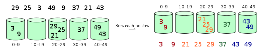
Bucket sort works as follows:
- Set up an array of initially empty “buckets”.
- Scatter: Go over the original array, putting each object in its bucket.
- Sort each non-empty bucket using bucket sort or other sorting methods.
- Gather: Visit the buckets in order and put all elements back into the original array.
Bucket sort is mainly useful when input is uniformly distributed over a range. The worst-case scenario occurs when all the elements are placed in a single bucket. The overall performance would then be dominated by the algorithm used to sort each bucket, which is typically $O(n^{2}) $ insertion sort, making bucket sort less optimal than $O(n\log_2n)$ comparison sort algorithms.
Examples:
| Input array | Suitable algorithm |
|---|---|
| 1, 1, 1, 2, 2, 3, 3, 3, 4, 5, 5 | Counting sort |
| 1, 995, 996, 996, 998, 999 | Radix sort |
| 1, 1, 1, 1, 1000, 1000, 1000 | Bucket sort |