Vector Semantics

The intuition is that perhaps there exists some multi-dimensional semantic space that is sufficient to encode all semantics of our words. Each dimension would encode some meaning. For instance, semantic dimensions might indicate tense (past vs. present vs. future), count (singular vs. plural), and gender (masculine vs. feminine).

Vectors for representing words are generally called embeddings, because the word is embedded in a particular vector space. Vector semantic models are extremely practical because they can be learned automatically from text without any complex labeling or supervision. Vector models of meaning are now the standard way to represent the meaning of words in NLP.

Words and Vectors

Vector or distributional models of meaning are generally based on a co-occurrence matrix, a way of representing how often words co-occur. However, these vectors are usually very sparse.

Vectors and Documents

In a term-document matrix, each row represents a word in the vocabulary and each column represents a document, which means a word vector is a row vector in the matrix and a document vector is a column. The term-document matrix has \(\mid\mathcal{V}\mid\) rows (one for each word type in the vocabulary) and \(\mid\mathcal{D}\mid\) columns (one for each document in the collection), where \(\mid\mathcal{V}\mid\) is the number of words in the vocabulary set $\mathcal{V}$, and \(\mid\mathcal{D}\mid\) is the number of documents in the documents set \(\mathcal{D}\).

As shown in the table below, The term-document matrix for four words in four Shakespeare plays. Each cell contains the number of times the (row) word occurs in the (column) document.

	As You Like It	Twelfth Night	Julius Caesar	Henry V
battle	1	0	7	13
good	114	80	62	89
fool	36	58	1	4
wit	20	15	2	3

Term-document matrices were originally defined as a means of finding similar documents for the task of document information retrieval. Information retrieval (IR) is the task of finding the document from the documents in some collection that best matches a query. For IR we also represent a query by a vector, also of length \(\mid\mathcal{V}\mid\), and we will need a way to compare two vectors to find how similar they are.

Later we will introduce the vector comparison processes: the tf-idf term weighting, and the cosine similarity metric.

Words as Vectors

As discussed above, we can represent a word as the row vector in term-document matrix. Similar words will have similar vectors because they tend to occur in similar documents.

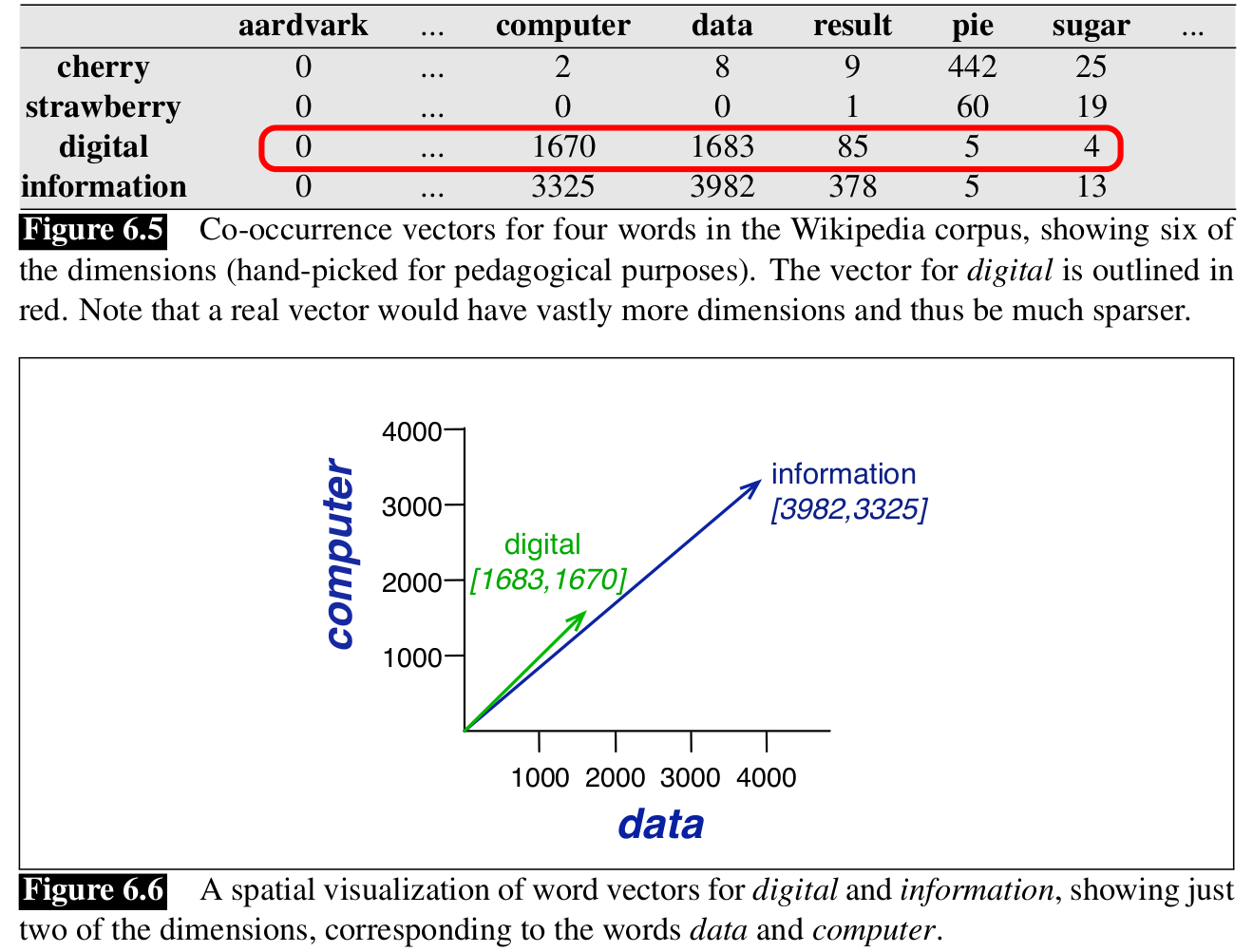
However, for word vector representation, rather than the term-document matrix, it is more common to use the word-word matrix (or term-term matrix, or term-context matrix). This matrix is of dimensionality \(\mid\mathcal{V}\mid \times \mid\mathcal{V}\mid\), and each cell records the number of times the row (target) word and the column (context) word co-occur in some context in some training corpus. The context could be a document, or a window around the word.

Figure 6.5 shows a simplified subset of the word-word co-occurrence matrix for these four words computed from the Wikipedia corpus.

Note that \(\mid\mathcal{V}\mid\), the length of the word vector, is generally the size of the vocabulary, usually between \(10,000\) and \(50,000\) words (using the most frequent words in the training corpus; keeping words after about the most frequent \(50,000\) or so is generlly not helpful). These vectors are usually very sparse since most of these numbers are zero, and there are efficient algorithms for storing and computing with sparse matrices.

Cosine for Measuring Similarity

By far the most common similarity metric for two vectors is the cosine of the angle between the vectors. The cosine similarity is based on the dot product (or inner product) operator:

\[\mathbf{a}^T \mathbf{b} = \sum_i a_ib_i.\]

Most metrics for similarity between vectors are based on the dot product, because it will tend to be high just when the two vectors have large values in the same dimensions. Alternatively, orthogonal vectors have a dot product of $0$, representing their strong dissimilarity.

This raw dot product, however, has a problem as a similarity metric: it favors long vectors. The vector length is defined as

\[\| \mathbf{a} \|_2 = \sqrt{\sum_i a_i^2}.\]

More frequent words have longer vectors, since they tend to co-occur with more words and have higher co-occurrence values with each of them. The raw dot product thus will be higher for frequent words. But this is a problem since we would like a similarity metric that tells us how similar two words are regardless of their frequency. The simplest way to modify the dot product to normalize for the vector length is to divide the dot product by the lengths of each of the two vectors.

This normalized dot product turns out to be the same as the cosine of the angle between the two vectors:

\[\cos (\mathbf{a}, \mathbf{b}) = \frac{\mathbf{a}^T \mathbf{b}}{\| \mathbf{a} \|_2 \| \mathbf{b} \|_2 } = \frac{\sum_i a_ib_i}{\sqrt{\sum_i a_i^2} \sqrt{\sum_i b_i^2}}.\]

TF-IDF

The intuition is that, some words (like the, it) are so unspecific that they occur in many documents and co-occur with almost all words, thus they are less informative than others. The TF-IDF algorithm penalize the term frequency by its unspecificity (document frequency). The TF-IDF is the product of term frequency (TF) and inverse document frequency (IDF).

Term Frequency (TF) measures how often does the term \(t\) occur in the document $d$. The importance does not increase linearly with the term frequency, so term frequency $\text{Count}(t)$ is often made smaller by log transformation, as \(\text{tf}(t,d) := \log\left(1+\text{Count}(t,d)\right),\)

where the logarithm base is usually \(10\).

Document frequency is \(\text{df}(t) := \frac{n(t)}{N}\), if term $t$ occurs in $n(t)$ out of $N$ documents. e.g. $\frac{1}{10}$ if “dog” occurs in only $1$ of $10$ documents. Then the Inverse Document Frequency (IDF) formula is defined as

\[\text{idf}(t) := \log \frac{1}{\text{df}(t)} = \log \frac{N}{n(t)}.\]

Higher of \(\text{idf}(t)\) means more specific of the term $t$.

Therefore, the TF-IDF is the product of TF and IDF:

\[\text{tfidf}(t,d) = \text{tf}(t,d) \times \text{idf}(t) = \log (1+\text{Count}(t,d)) \times \log \frac{N}{n(t)}.\]

Overall, TF is big when term $t$ occurs often in document, and IDF is big when term $t$ does not occur in many other documents.

Cosine similarity works better with TF-IDF values than with original frequencies.

Reference:

Jurafsky, D., Martin, J. H. (2009). Speech and language processing: an introduction to natural language processing, computational linguistics, and speech recognition. Upper Saddle River, N.J.: Pearson Prentice Hall.